Function Generator vs Arbitrary Waveform Generator: What You Are Buying
Three names, two architectures: how DDS and point-by-point playback differ, what the labels hide, and how to read the architecture off a datasheet.
By YDT Editorial18 min read
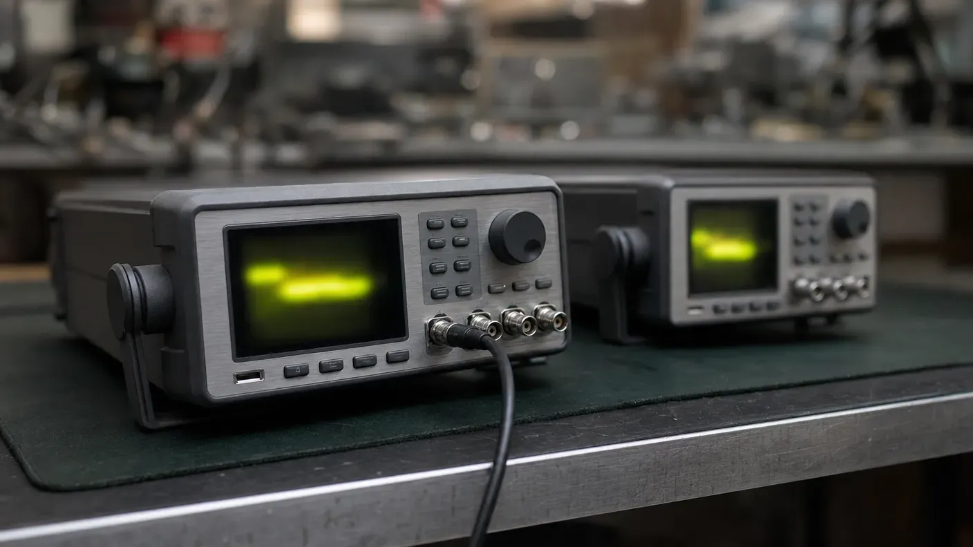
Two datasheets are open on the bench. One instrument calls itself an arbitrary function generator, the other an arbitrary waveform generator, and nothing in either document tells you whether that difference is a marketing choice or an engineering one. Or the instrument is already on the bench, its front panel offers an arbitrary mode, and a waveform loaded into it is not coming back out the way it went in.
Both problems have one root: three names circulate for instruments built on two architectures, and the names do not map onto the architectures consistently from vendor to vendor. This article will not tell you which model to buy and will not declare either architecture the better one. It gives you the mechanical difference between the two ways a generator can read waveform points out of memory, the vocabulary map that lets you work out which one a datasheet is describing, and what each choice does to a signal whose detail is not periodic.
What the Label on the Front Panel Does Not Tell You
The purchasing question usually gets settled before this one arrives. It turns on a single criterion: is the signal you need one of the standard periodic shapes — sine, square, triangle, pulse — or does it have to be defined point by point, because it is a captured real-world signal, a modelled pulse or a modulation pattern? That branch decision, and everything a purchase depends on around it, belongs to a specification-led guide to choosing a signal generator and is not re-derived here.
The trouble is that the criterion picks a family, and the family names are not reliable identifiers of what is inside a given box. Three terms are in use for instruments built on two distinct architectures — function generator, arbitrary function generator, arbitrary waveform generator — and which term lands on which architecture varies by vendor. Microwaves & RF applies “arbitrary function generator” to direct digital synthesis instruments. National Instruments ties the plain term “function generator” to DDS. Keysight markets its arbitrary waveform generator line under the TrueForm name, which Keysight characterises as its non-DDS architecture.
So an engineer holding two datasheets is holding two vocabularies, and no amount of care with the word arbitrary resolves it. What does resolve it is the mechanism: how the instrument reads stored points out of memory. That mechanism is also what decides whether your waveform survives the trip to the output connector.
Three Names, Two Architectures
Start with what each source actually says, in its own words, because the disagreement is the point.
Microwaves & RF treats the two terms as synonyms: “a DDS, also known as an arbitrary function generator (AFG), reads waveform samples stored in memory using a phase accumulator at a fixed clock rate.” In that usage, AFG is DDS.
National Instruments’ terminology page states that function generators “employ direct digital synthesis (DDS) to precisely generate standard waveforms that are repetitive in nature, including sine, TTL, square, and triangular waveforms,” that those standard shapes are generally pre-defined in memory, and that the instrument additionally carries a small memory depth allowing the user to define one period of their own waveform. Its arbitrary waveform generator family is characterised the other way: deep onboard memory — 256 MB to 1 GB on the PXIe-5433 — sufficient to store several waveform segments plus instructions on how to sequence them and how many times to output each one.
Keysight adds a third convention, an architecture brand. Microwaves & RF refers to “the 33600A Series TrueForm AWGs from Keysight Technologies” — sinewaves to 120 MHz, pulses to 100 MHz, sampling rates to 1 Gsample/s, 14-bit amplitude resolution, up to 64 Msample/channel of arbitrary memory. Keysight’s own characterisation of TrueForm as a non-DDS architecture is attributed here rather than independently verified: the Keysight pages carrying it could not be opened for this article.
Put the three conventions side by side and the conclusion is unavoidable. There is no industry-wide mapping from name to architecture. “Arbitrary” on one datasheet can name a capability of a different shape from “arbitrary” on another, and the reader has to map each vendor’s term onto the mechanism themselves.
| Term as written | Usage on record | Architecture it usually indicates |
|---|---|---|
| Function generator | NI ties it to DDS generation of standard repetitive shapes, with small memory for one user-defined period | Phase accumulator (DDS) |
| Arbitrary function generator (AFG) | Microwaves & RF uses it as another name for a DDS instrument | Phase accumulator (DDS) |
| Arbitrary waveform generator (AWG) | NI ties it to deep memory with segment sequencing; Microwaves & RF describes point-by-point conversion on a variable reference clock | Point-by-point playback |
| Vendor architecture name (e.g. Keysight TrueForm) | Branding on Keysight’s AWG line; characterised by Keysight as non-DDS (attributed, not verified here) | Point-by-point playback |
Two Ways to Read the Same Memory
Strip both instruments down and they look alike: digital waveform points held in memory, a converter turning those points into volts. What differs is the read pattern, and setting the two patterns against each other is where the whole comparison lives.
The accumulator architecture clocks its memory at a fixed rate. A phase accumulator advances by a programmed phase increment on each clock cycle, and its value selects which stored phase point gets read. Microwaves & RF describes the consequence plainly: to change frequency, the instrument reads samples for the phase angles of the waveform, leaving gaps between phase samples, and the number of sampled phase points together with the size of the increments between phase angles determines the length and frequency of the waveform. Larger phase increments generate higher frequencies. Because the increment is a register value rather than an oscillator setting, the frequency change is instant — and a DDS uses fewer samples than an AWG to construct its output waveform.
Point-by-point playback inverts both halves. The same source describes an AWG converting waveform samples stored in memory to output “in a continuous, point-by-point fashion, using a variable-frequency reference-clock oscillator”: one sample converted per clock cycle, output frequency determined by the reference clock’s frequency, faster clock rates producing higher output frequencies — and the waveform shape remaining constant regardless of the clock frequency.
One sentence holds the difference. The accumulator varies the address step and leaves the clock alone; playback varies the clock and leaves the address step alone. Everything else in this article is a consequence of that.
This immediately explains something that confuses readers coming from the front panel: for a sinewave, the two architectures are indistinguishable at the output. Microwaves & RF says why — signals with continuous shapes, such as sinewaves, are relatively unaffected by large increments between phase angles. A shape that repeats is still fully described by the reduced set of phase samples, so the points an accumulator steps over carry nothing the remaining points do not already imply. Skipping is not an approximation there; it is redundancy elimination.
What the Skipped Points Take With Them
The redundancy argument fails the moment the interesting part of the waveform stops repeating. Microwaves & RF is explicit: signals with discontinuous shapes, anomalies or transient characteristics — fast pulse rise and fall times being the named case — can be difficult to create accurately with a DDS. And it names the failure mode rather than leaving it as “reduced fidelity”: samples representing transient events that are part of a waveform may not be triggered at a given clock rate and by a given number of samples, so the output waveform is not truly representative of the original sampled waveform.
The useful working test is not how complicated your waveform looks. A heavily harmonic but strictly repeating shape is fine; a mostly flat trace with one glitch in it is not. The property to check is the periodicity of the detail you care about: whatever lives in the repeating portion survives accumulator skipping, and whatever does not — anomalies, transients, single events, the fast edge you are trying to stress a receiver with — is precisely what the skipped points take away.
What Happens to a Waveform You Download Into a Function Generator
This is the second reader’s problem, and it is the part of the comparison that almost nothing on the subject states. You define a shape in software, download it into the instrument, and the output is recognisably your waveform with the sharp features rounded or missing. Nothing malfunctioned.
Keysight’s account of what a DDS instrument does with a downloaded record explains it, and the attribution matters: this reaches us through a Keysight page that was not accessible for this article, so it travels on that attribution rather than as a fresh verification. The description is that a downloaded waveform is not played point by point as received, but stretched by interpolation to fill the memory the architecture requires. On the 33220A, downloaded points are expanded to 16K or 64K whatever the original length of the waveform you sent.
Read that against point-by-point playback, where stored points are converted in the order they occupy memory, and the vocabulary problem from the first section stops being cosmetic. On the accumulator instrument, “arbitrary” means you may define a shape, which the instrument will resample to a length it chooses. On the playback instrument, it means the points you wrote are the points that come out. Both statements are legitimately printed as “arbitrary waveform capability”, and only the second one guarantees that a downloaded record survives as loaded.
Where the Two Datasheets Actually Diverge
Neither architecture is a compromised version of the other. Each spends something to buy something, and the specification pages show where.
Frequency resolution. Microwaves & RF states that DDS sources running at high clock frequencies are typically capable of higher-resolution frequency tuning than AWG sources. The reason sits in the arithmetic of clock-based synthesis, which the same source works out: the number of frequency points available from the sample clock determines frequency precision, so an AWG built on a standard 10 MHz clock oscillator and designed for a 100 MHz maximum output has twice the frequency resolution of one designed for 200 MHz on the same clock — the oscillator’s limited set of frequency points is being spread across twice the bandwidth. Tuning resolution on a playback instrument is therefore partly a design-bandwidth decision, not just a clock-quality one.
National Instruments defines spurious-free dynamic range as the usable dynamic range before spurious noise interferes with or distorts the fundamental: the ratio between the fundamental signal and the largest harmonically or non-harmonically related spur from DC to half the sampling rate, most commonly in dBc. An SFDR of about 70 dBc means the worst spur sits 70 dB below the carrier. Where tuning resolution and spectral purity have to be weighed against each other for a purchase, that trade-off is developed in the signal generator selection guide.
Sample rate and memory depth, on the generation side, bound what a played waveform can contain and how long it can run. NI defines sample rate as the rate at which digital data is transferred from memory to the DAC, and states the constraint directly: a digital waveform must be updated at least twice as fast as the highest frequency of the desired signal to be generated accurately, with a higher sample rate capturing more waveform detail. Memory depth then sets how long a unique waveform runs before repeating — NI’s worked case is 256 million samples at 100 MS/s giving 2.56 s of play time. The coupling matters specifically for playback instruments: because they raise output frequency by clocking through memory faster, the same stored record plays for less time at higher output frequency.
Vertical resolution binds on both architectures and the sources describe no architectural difference in it. It is the DAC’s bit count against the selected range: the smallest step is the peak-to-peak range divided by 2^N levels. NI’s examples on a 0–10 V range — a 3-bit converter dividing the range into eight levels and unable to produce differences smaller than 1.25 V, a 16-bit converter with 65,536 levels resolving about 153 µV — make the lever obvious. It is range and offset matching, not architecture: a 1 V peak-to-peak sine sitting between 1 V and 2 V wants the 1 V range with a 1.5 V offset.
| Specification | Phase accumulator (DDS) | Point-by-point playback |
|---|---|---|
| Frequency resolution | Typically higher-resolution tuning when running at high clock frequencies | Bounded by the frequency points the sample clock can produce, spread over the design bandwidth |
| Frequency change | Essentially instantaneous — a changed phase increment | Requires moving the reference-clock frequency |
| Fidelity at higher output frequency | Stored points are stepped over; continuous shapes survive, transients may not be triggered | Waveform shape remains constant regardless of clock frequency |
| Downloaded custom waveform | Expanded by interpolation to the memory size the architecture requires (Keysight, attributed) | Converted in the order the points occupy memory |
| Memory figure | On NI function generators, small enough for one user-defined period — not a DDS-wide figure | Deep — 256 MB to 1 GB on the PXIe-5433, with segment sequencing (NI) |
Instruments That Are Both
If the two architectures answer different questions, the obvious design move is to fit both. Microwaves & RF notes exactly that: DDS-based sources are often included in AWG designs “to provide the benefits of both technologies within a single package,” the stated motivation being the higher-resolution frequency tuning DDS typically offers.
The Tektronix AWG4000 is the source’s worked example — an instrument that “functions as both an AWG and a DDS.” In basic DDS mode it operates at 2.5 Gsamples/s with 14-bit resolution and 16 kpoints of arbitrary waveform memory, its two channels each able to output sinewaves to 600 MHz.
Read those numbers again with the qualifier attached: they are the DDS-mode figures, distinct from the same instrument’s AWG-mode specification. That is the practical trap in a dual-architecture datasheet. A specification on such a page belongs to an operating mode, not to the instrument, and a buyer who lifts the headline sample rate or memory figure out of one mode and plans to work in the other has compared numbers that were never going to hold together.
Reading the Architecture Off a Datasheet
With the name unreliable, the datasheet is still the evidence — it just has to be read for mechanism rather than for family. Four observations, in rough order of how decisive they are:
- The clock. A datasheet describing generation from memory at a fixed clock, with output frequency set by a phase increment or tuning step, is describing the accumulator architecture. One describing output frequency set by varying the reference or sample clock is describing point-by-point playback.
- The memory figure. A number that downloaded points are expanded to fill — Keysight’s 33220A expanding downloads to
16Kor64Kis the worked case, on the Library’s attribution — indicates the DDS treatment of downloaded waveforms. A depth figure that supports play-time arithmetic, depth divided by sample rate, indicates points played as stored. - The naming convention. “Arbitrary function generator” in Microwaves & RF’s usage indicates DDS. Where a vendor explicitly characterises its own architecture, that characterisation is usable evidence — Keysight’s TrueForm branding, characterised by Keysight as non-DDS, is the example, and it is attributed rather than verified here.
- Explicit architecture statements. Some vendors name the architecture outright, in which case there is nothing to infer.
What the test does not license is as important as what it does. Each observation identifies an architecture only where the datasheet states it: silence about phase increments or about a variable clock proves nothing, because no vendor is obliged to disclose architecture at all. The memory observation distinguishes the treatment of downloaded waveforms, not the generation of standard periodic shapes — for those, the two architectures produce indistinguishable output, so no amount of datasheet reading will separate them on a sinewave specification. And this reading test is engineering practice assembled from the mechanism descriptions, not a vendor-published procedure.
Which One Your Bench Needs
Microwaves & RF puts the conclusion in one line worth keeping: both types of signal source are widely used in test and system applications, chosen for their different performance capabilities. Not ranked — chosen.
The accumulator architecture buys essentially instantaneous frequency changes, typically higher-resolution frequency tuning, and advanced output functions such as digital modulation and frequency hopping. That suits stimulus work where the wanted signal is one of the standard periodic shapes, and it suits anything frequency-agile, where the ability to jump frequency on a register write is the specification that matters.
Point-by-point playback buys, in the same source’s words, “much greater control and precision for its generated waveforms,” with the shape held constant regardless of clock frequency, and — per NI — deep memory holding several waveform segments together with sequencing instructions. That suits work whose detail is not periodic: replaying a captured real-world signal, a modelled pulse, a modulation pattern built in software.
Settle it on your own stimulus rather than on the instrument. Write down the signal you actually have to produce and ask whether its informative detail repeats. If it does, the accumulator architecture will reproduce it and hand you tuning agility as a bonus. If it does not — if the point of the signal is an edge, a glitch, a one-off transient or a sequence — then every point has to be played, and only one of the two architectures promises that. Converting that answer into the rest of a specification list, amplitude and load, bandwidth against sample rate, resolution and play time, is the job of choosing a signal generator by specification.
Frequently Asked Questions
Is a function generator an arbitrary waveform generator?
Generally no, even where its front panel offers an arbitrary mode. National Instruments ties the function generator family to direct digital synthesis of standard repetitive shapes with a small memory allowing the user to define one period, while it characterises arbitrary waveform generators by deep memory holding several waveform segments plus sequencing instructions.
What is a true arbitrary waveform generator?
One that converts its stored waveform samples to output in a continuous, point-by-point fashion using a variable-frequency reference-clock oscillator, one sample per clock cycle. Output frequency comes from the clock rate, and the waveform shape remains constant regardless of that rate.
Why does a waveform I downloaded not come out the way I loaded it?
On a DDS instrument, Keysight's account is that downloaded points are not played as received but stretched by interpolation to fill the memory the architecture requires; on the 33220A they are expanded to 16K or 64K points whatever the original length. That figure travels on Keysight's attribution rather than as an independently verified measurement.
Can one instrument be both a DDS and an AWG?
Yes. Microwaves and RF notes that DDS sources are often included in AWG designs to provide the benefits of both technologies in one package, and cites the Tektronix AWG4000 as functioning as both, with figures published per operating mode.
How do I tell from a datasheet which architecture is inside?
Check whether the sample clock is described as fixed with output frequency set by a phase increment, or as variable, and whether the memory figure supports play-time arithmetic or is a size that downloaded points are expanded to fill. The absence of either description proves nothing, since vendors are not obliged to disclose the architecture.
Filed under
Related articles
Electronics23 min read
How to Choose a Signal Generator: Getting the Signal You Asked For
How to turn a required stimulus into datasheet requirements: the load the instrument assumes, bandwidth against sample rate, reconstruction and vertical resolution.
Electronics22 min read
How to Choose a Multimeter: A Specification-Led Buying Guide
Choose a multimeter by the errors it introduces: burden voltage, input loading, AC bandwidth, safety category and accuracy on the reading you actually take.
Electronics16 min read
How to Use a Thermal Camera: Getting Readings You Can Trust
A thermal camera always shows a number. Learn the checks — emissivity, reflected temperature, focus and spot size — that decide whether it is a measurement.
Electronics21 min read
FFT on Oscilloscopes: Principles, Setup, and Interpretation
How an oscilloscope's FFT function works, how sample rate, record length and window functions affect the result, and how to interpret an FFT spectrum in engineering work.