FFT on Oscilloscopes: Principles, Setup, and Interpretation
How an oscilloscope's FFT function works, how sample rate, record length and window functions affect the result, and how to interpret an FFT spectrum in engineering work.
By YDT Editorial21 min read
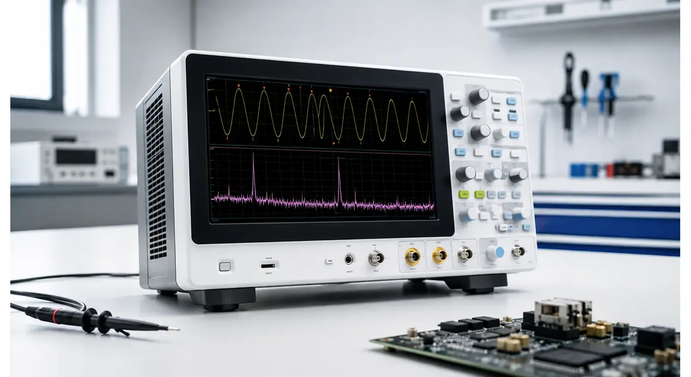
A 12 V rail measures 40 mV of ripple. The trace is a fuzzy band with some periodic structure buried inside it, and nothing on the screen tells you where it comes from. Is it the switching regulator? Line ripple making it through the bulk capacitor? A clock coupling into the feedback network? In the time domain everything arrives summed together, and the display gives you no way to separate the contributors.
The frequency domain does. The same acquisition, transformed, places a 340 kHz switching fundamental, a 120 Hz line component and a clock spur in three different parts of the screen, with amplitudes you can compare directly. You stop guessing and start reading a list of suspects. That transformation is what the FFT function on a digital oscilloscope provides.
This guide covers what the FFT actually computes, the settings that decide whether the result is trustworthy, how to read a spectrum the way an experienced engineer does, and where the oscilloscope’s limits end and a spectrum analyzer’s job begins. It is part of our complete Test & Measurement guide, which covers the rest of the bench.
What Is FFT on an Oscilloscope?
Frequency-domain analysis vs. time-domain analysis
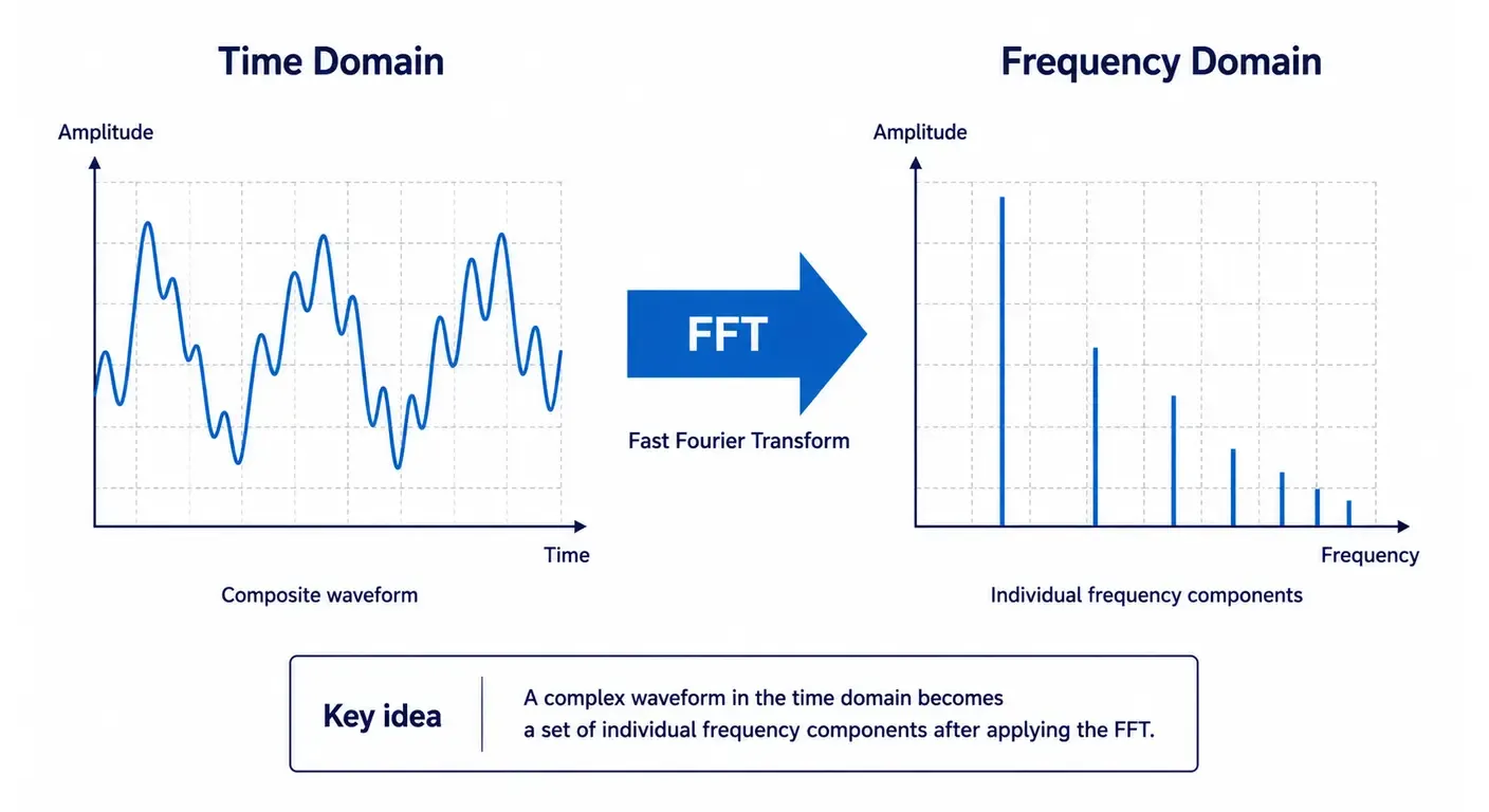
The standard oscilloscope display answers one question: what does this signal do over time. The frequency domain answers a different one: what is this signal made of. Any repetitive waveform can be described as a sum of sinusoids with different frequencies, amplitudes and phases. The time-domain view shows their sum; the frequency-domain view shows the individual contributors.
Think of a band playing in a room. Your ear hears one combined sound — that is the time domain. The frequency domain is the list of which instruments are playing and how loudly, which is far more useful when one of them is out of tune.
The distinction is practical rather than philosophical. “40 mV of ripple” is a single number describing a total disturbance. A spectrum showing 28 mV at 340 kHz and 9 mV at 120 Hz points at two different components on the board and two different design decisions.
What the Fast Fourier Transform computes
The FFT is an efficient algorithm for computing the Discrete Fourier Transform of a finite block of samples. Given N samples acquired at a sample rate of Fs, it returns a set of frequency bins spanning DC to Fs/2, each holding the amplitude and phase of one narrow slice of the spectrum. For a real-valued input signal, only the first N/2 bins carry unique information.
The algorithm’s value is purely computational. A direct DFT costs on the order of N² operations; the Cooley-Tukey approach reduces this to N log N, which is what makes the transform practical on an embedded oscilloscope processor. Many implementations require N to be a power of two, which is why FFT record lengths are usually offered as a fixed list rather than a continuous range.
One framing is worth carrying through the rest of this article. The oscilloscope is not listening to your circuit continuously the way a radio receiver does. It records a short clip, analyzes that clip, then discards it and records another. Everything the FFT tells you is inferred from one finite recording — and almost every artifact and limitation described below follows from the word “finite.”
Why FFT is integrated into digital oscilloscopes
Because the samples are already in memory. Once a digital oscilloscope has digitized a waveform, producing a spectrum is a mathematical operation on data the instrument already owns. That gives it three advantages a swept analyzer cannot match: the spectrum is time-correlated with the waveform that produced it, it works on single-shot and transient events, and it costs nothing extra.
The second point matters more than it sounds. When a fault appears once every few minutes, you can trigger on it, capture it, and inspect its frequency content afterwards — something a swept instrument, which only ever looks at one narrow slice of the spectrum at a time, will simply miss.
Why Engineers Use FFT Measurements
In practice, the FFT earns its place on the bench in a handful of recurring situations.
Detecting unwanted frequency components. A signal that looks acceptable in the time domain may carry low-level periodic content the vertical scale cannot show. A 5 mV interferer riding on a 3.3 V logic supply is invisible at 1 V/div, but stands out clearly in a spectrum.
Harmonic analysis. Distortion mechanisms in amplifiers, converters and rectifiers express themselves as energy at integer multiples of the fundamental. The relative heights of the second, third and fifth harmonics often identify the mechanism — symmetric clipping produces odd harmonics, asymmetric distortion produces even ones.
Noise characterization. The spectrum separates broadband noise, which raises the whole floor, from narrowband interference, which produces discrete peaks. That distinction tells you whether you are chasing a thermal limit or a coupling path — two very different afternoons.
Switching power electronics. Converters produce a dense harmonic comb built on the switching frequency. FFT lets you confirm the switching frequency, watch for subharmonic behavior, and see whether high-order harmonics land where they will cause trouble.
Audio and vibration analysis. Mechanical systems produce characteristic spectral signatures. Rotational imbalance, bearing defects and gear-mesh frequencies each occupy predictable positions relative to shaft speed.
EMI pre-compliance troubleshooting. Long before a formal test campaign, FFT on a near-field probe or a supply rail identifies which emitter is responsible for a given frequency — the question formal EMC data alone rarely answers.
How FFT Works Inside an Oscilloscope
Knowing what the FFT is good for is one thing; knowing when to believe it requires understanding where the numbers come from.
Everything begins with a normal acquisition. The analog front end conditions and band-limits the signal, the ADC digitizes it at the current sample rate, and samples fill the acquisition memory. The FFT then operates on that stored record; no separate hardware path is involved.
Two relationships govern the result. The span — the highest frequency the transform can represent — is Fs/2, the Nyquist frequency. The bin width, which sets frequency resolution, is:
Δf = Fs / N = 1 / Twhere N is the number of samples transformed and T is the duration of the record. The second form is the one to internalize: frequency resolution is determined by how long you observed the signal, not by how fast you sampled it. Sampling faster with the same memory buys span and costs resolution.
This is where most people get caught. Acquire 100 kpts at 250 MSa/s: the record covers 400 µs, so the bin width is 2.5 kHz and the span reaches 125 MHz. Two signals 1 kHz apart fall inside the same bin and appear as one peak — and no amount of zooming will separate them, because the information was never captured. Resolving them requires a record of at least 1 ms, which at the same sample rate means 250 kpts. That is why memory depth matters as much for spectral work as it does for long time-domain captures.
Dynamic range, meanwhile, is set primarily by the ADC. The theoretical signal-to-noise ratio of an ideal N-bit converter driven by a full-scale sine wave is approximately 6.02N + 1.76 dB — roughly 50 dB for 8 bits, roughly 74 dB for 12 bits. Real front ends achieve fewer effective bits than their nominal resolution, particularly at high frequencies.
Factors That Influence FFT Accuracy
Beyond those two governing equations, four practical factors decide whether the spectrum in front of you deserves to be trusted.
The sample rate must be chosen deliberately, not inherited. At slow time base settings, most oscilloscopes quietly reduce the sample rate to avoid filling memory. You widen the time base to catch a slow load transient, the instrument drops from 500 MSa/s to 50 MSa/s without announcing it, and every real signal above 25 MHz folds back into the display as a false peak.
Analog bandwidth still applies. The FFT cannot recover what the front end already attenuated. A harmonic sitting near or above the instrument’s -3 dB point is displayed below its true amplitude, and one well beyond it may not appear at all. When measuring harmonic content, confirm that the highest harmonic of interest sits comfortably inside the oscilloscope’s bandwidth — a useful working rule is headroom of three to five times the fundamental.
Quantization noise sets a floor you cannot escape. Using only two of eight vertical divisions wastes most of the ADC range and raises the effective noise floor by roughly 12 dB. Scaling the waveform to fill the screen is not cosmetic; it directly buys dynamic range.
External noise adds to that floor. Ground-lead pickup, nearby switching supplies and unshielded leads all contribute. A spectrum taken with a 15 cm ground lead and one taken with a spring-tip ground on the same node can differ by tens of dB in the tens-of-megahertz region.
FFT Window Functions Explained
Why spectral leakage occurs
The transform assumes the captured record repeats forever. If the record does not contain a whole number of signal cycles, its end does not match its beginning, and the implied repetition contains a discontinuity. That discontinuity is broadband, so energy from one tone smears into neighboring bins — the effect known as spectral leakage.
Picture splicing a length of recording tape into a loop. If the ends do not match, the splice produces a click on every rotation, and that click contains frequencies that were never in the original material. Your FFT displays those invented frequencies alongside the real ones.
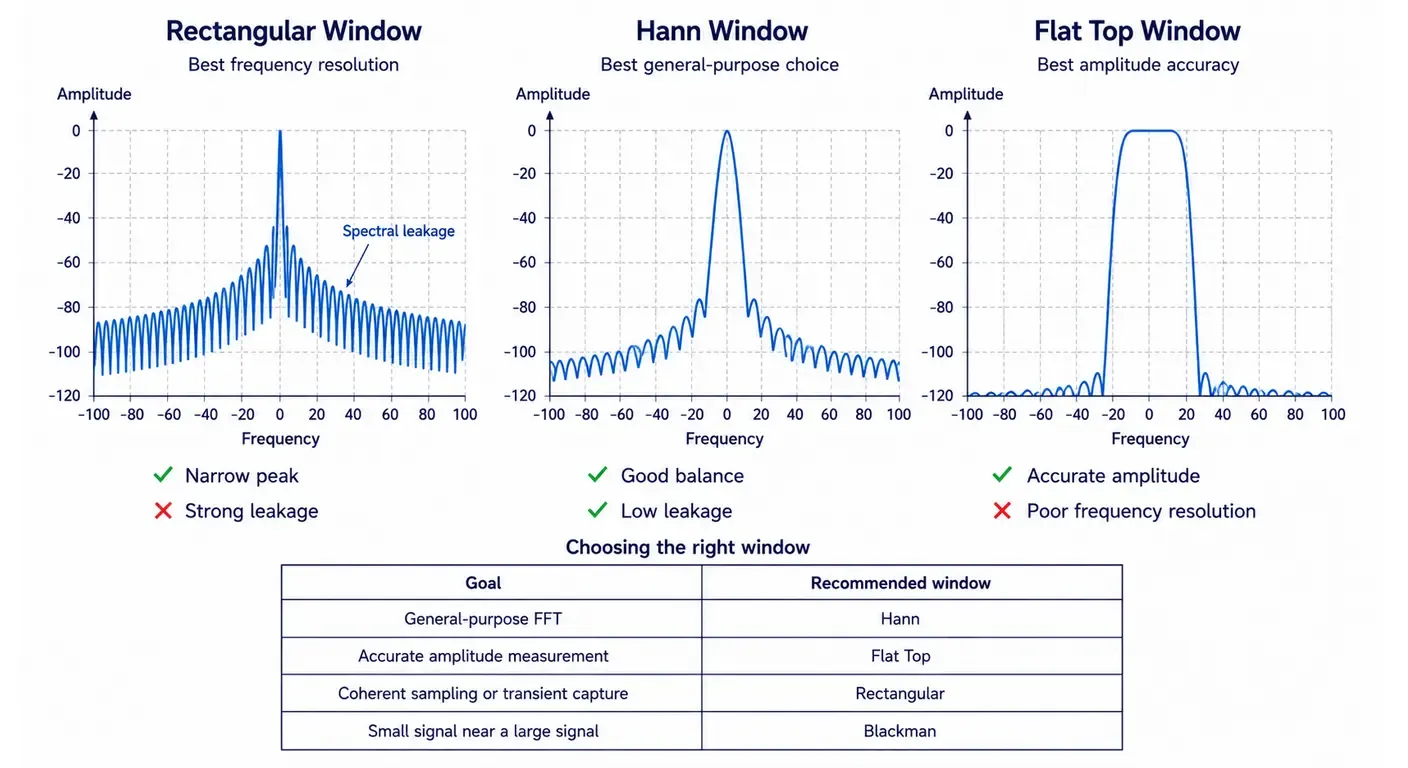
This is not an academic concern: leakage skirts from a large signal routinely bury the small one you were looking for. A window function fixes it by tapering the record smoothly to zero at both edges, removing the discontinuity — but it also widens the apparent peak and reduces the accuracy of its measured amplitude. Every window is simply a chosen position on that trade-off.
Typical characteristics of common FFT windows. Main-lobe widths are null-to-null and approximate; exact values depend on the implementation.
| Window | Main-lobe width (bins) | Highest side lobe | Worst-case amplitude error | Best suited to |
|---|---|---|---|---|
| Rectangular (none) | 2 | -13 dB | 3.9 dB | Transients fully contained in the record; signals sampled coherently |
| Hann | 4 | -31 dB | 1.4 dB | General-purpose analysis of continuous signals and noise |
| Hamming | 4 | -43 dB | 1.8 dB | Separating closely spaced tones of similar amplitude |
| Blackman | 6 | -58 dB | 1.1 dB | Finding small signals close to a much larger one |
| Flat Top | ≈9 | ≈ -70 dB | under 0.1 dB | Accurate amplitude measurement of well-separated tones |
Choosing the appropriate window
The choice follows from what you are trying to learn. If the question is how much, use Flat Top: it measures amplitude to a fraction of a decibel at the cost of a wide, blunt peak. If the question is at what frequency, or is that one signal or two, use a narrower window — Hann, Hamming or Blackman. For an impulse or a decaying transient that starts and ends inside the record, use Rectangular; there is no discontinuity to suppress, and tapering would only destroy information.
The failure mode is easy to reproduce. An engineer measuring line-frequency content picks Flat Top for its amplitude accuracy, then tries to tell a 50 Hz component from a 60 Hz one in the same record. With a 100 ms acquisition the bin width is 10 Hz, and the Flat Top main lobe spans roughly nine bins — the two tones merge into a single broad hump, and the measurement quietly says nothing. Switching to Hann resolves them immediately, at the cost of about 1.4 dB of amplitude uncertainty. The reverse mistake is just as common: using Rectangular to hunt for a harmonic 60 dB below the fundamental, where leakage buries it completely.
How to Configure FFT on an Oscilloscope
With the theory settled, the setup becomes mechanical — provided you work in the right order. The settings interact, and adjusting them out of sequence usually means adjusting them twice.
- Select the source channel and probe correctly. Use the shortest possible ground connection and confirm probe compensation. For rail measurements, AC coupling with vertical offset lets you expand the vertical scale without losing the trace. See the oscilloscope probe guide for connection techniques that preserve high-frequency content.
- Set the required frequency resolution first. Decide the smallest frequency spacing you must resolve, then set the record duration to at least 1/Δf. This is a time base decision, not an FFT decision.
- Set the sample rate for the span you need. The highest frequency of interest must sit below Fs/2, with margin. If the instrument reduces sample rate automatically, override it.
- Maximize record length. Deep memory is what lets steps 2 and 3 be satisfied at the same time. Manual memory selection is almost always better than automatic for spectral work.
- Choose the window according to whether amplitude or frequency separation matters more.
- Set the amplitude scale. Logarithmic scaling in dBV or dBm suits comparisons between components of very different sizes; linear V RMS is easier when the amplitudes are similar. If the instrument offers dBm, check the reference impedance it assumes — on a 1 MΩ input, a dBm reading only means something if the source is genuinely terminated in 50 Ω.
How to Interpret an FFT Display
A correctly configured spectrum is only useful if you can read it, and reading one is largely a matter of recognizing a small vocabulary of features.
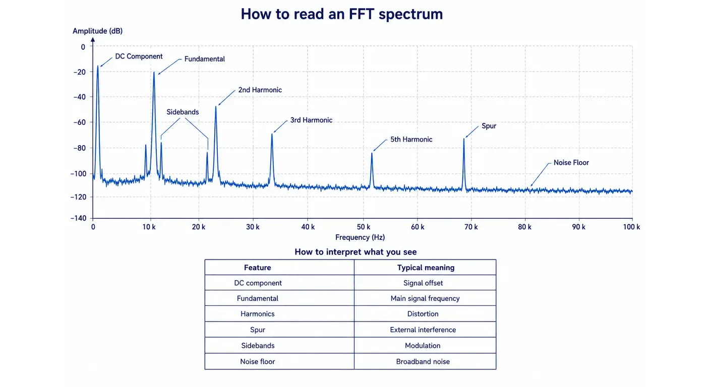
The fundamental is normally the largest peak and sets the reference for everything else. Harmonics appear at exact integer multiples of it, and their pattern is diagnostic: symmetric clipping favors odd harmonics, asymmetric distortion produces strong even ones.
Spurs are discrete peaks with no harmonic relationship to the fundamental. They almost always come from somewhere else — a switching converter, a nearby clock, or a coupling path into your own measurement setup.
Sidebands are pairs of peaks placed symmetrically either side of a carrier, and they mean something is modulating that carrier. Their offset names the culprit directly. On a motor drive showing a vibration nobody could explain, sidebands sitting 24 Hz either side of the drive fundamental point at the shaft rotation rate rather than the inverter; on a converter, sidebands 120 Hz out indicate line-frequency modulation of the control loop.
The noise floor is the broadband level between peaks. Its absolute value depends on record length and averaging, so treat it as a basis for comparison between measurements taken with identical settings, not as an absolute figure. A DC component at the left edge is normal with DC coupling and simply reflects the signal’s average value.
Aliasing artifacts are the most dangerous feature of an FFT display, because they look exactly like real signals. A component at frequency f above Nyquist appears at Fs - f. Sampling at 100 MSa/s, a genuine 60 MHz emission is drawn at 40 MHz — a frequency at which nothing in your circuit operates, which is precisely why engineers lose hours hunting for its source.
Practical Engineering Applications
That same vocabulary reappears across very different circuits.
Power supply ripple analysis. A rail’s total ripple is a single number; its spectrum is a diagnosis. Energy at the switching frequency points to output filtering, energy at 100 or 120 Hz points to bulk capacitance or rectifier behavior, and content well above the switching fundamental usually means switch-node ringing is coupling onto the output.
Switching regulator debugging. A peak at exactly half the switching frequency is the classic signature of subharmonic oscillation in peak-current-mode control running above 50 % duty cycle with inadequate slope compensation. In the time domain it looks like alternating wide and narrow pulses, easy to dismiss as jitter; in the frequency domain it is unmistakable.
Motor drive diagnostics. On the output side, the spectrum separates the PWM carrier from the drive fundamental. On the input side, a six-pulse rectifier produces a characteristic pattern at the 5th, 7th, 11th and 13th harmonics of the line frequency — the orders that dominate installation-level power quality problems.
Clock signal analysis. FFT shows harmonic content, spurs coupling in from other rails, and sidebands produced by periodic jitter. It also makes spread-spectrum clocking obvious: peaks broaden and flatten instead of standing sharp.
Audio amplifier testing. Harmonic ratios reveal distortion mechanisms quickly. Recognize the limit, though: an amplifier specified below 0.01 % THD sits beneath what an 8-bit front end can credibly resolve, even with averaging. FFT identifies the character of the problem here; an audio analyzer quantifies it.
Sensor signal evaluation. With accelerometers, load cells and similar low-level sensors, FFT separates the mechanical signature from mains hum and its harmonics — often the difference between a real measurement and a grounding problem.
Oscilloscope FFT vs. Spectrum Analyzer
Which raises the obvious question: if the oscilloscope can do all this, when is a spectrum analyzer still worth carrying to the bench?
Pros
- Captures the entire span simultaneously, so transient and intermittent events are not missed between sweeps
- Spectrum is time-correlated with the waveform, allowing a peak to be traced back to the moment that produced it
- Works on single-shot events, which a swept analyzer cannot capture at all
- Multiple channels can be analyzed from the same triggered acquisition
- Requires no additional instrument, cabling or setup time
Cons
- Dynamic range is limited by an 8- or 12-bit ADC rather than a dedicated low-noise receiver
- Sensitivity is far lower, so small signals near a large one are difficult to resolve
- Amplitude accuracy is typically a few percent, not a fraction of a decibel
- No preselection or tracking filter, leaving the front end exposed to out-of-band energy
- No resolution bandwidth control or standards-defined detectors
The analyzer wins whenever the measurement depends on sensitivity, dynamic range or traceable amplitude: formal EMC work requiring quasi-peak or average detectors, phase noise characterization, low-level spurious searches, and any harmonic measurement where the harmonic of interest lies 80 dB or more below the fundamental. The practical division of labor is simple — use the oscilloscope’s FFT to find and identify the problem on the bench, and a spectrum analyzer or EMI receiver to quantify and document it.
Common Measurement Errors
Almost every misleading spectrum comes from the same short list, and all of these mistakes look perfectly plausible on screen.
Selecting a window without a reason. Flat Top merges closely spaced tones; Rectangular buries small signals under leakage from large ones.
Accepting whatever sample rate the time base chose. A slow time base can drop the sample rate far below the front-end bandwidth, and everything above the new Nyquist frequency folds into the display.
Insufficient frequency resolution. Two peaks inside one bin are one peak. If a component you expected is missing, check the bin width before concluding it is not there.
Ignoring the probe. A long ground lead forms a resonant loop with the probe capacitance, producing a peak in the tens of megahertz that belongs entirely to the measurement setup. Probe bandwidth and loading also attenuate the high-order harmonics you may be trying to measure.
Misreading amplitudes. A tone that does not fall exactly on a bin center is displayed low — up to 3.9 dB with a Rectangular window. Confusing dBV with dBm, or reading dBm on a high-impedance input, produces errors of similar size for entirely different reasons.
Trusting a peak observed once. Before acting on an unexpected frequency component, reproduce it under at least one changed acquisition setting.
Best Practices for Reliable FFT Measurements
Work backwards from the requirement: define the frequency resolution you need, set the record duration accordingly, then confirm that the sample rate covers your span and that memory depth supports both at once. Use the deepest available record; it improves resolution and lowers the displayed noise floor at the same time.
Fill the vertical range without clipping, and use averaging when hunting for components near the noise floor — with a stable trigger on a repetitive signal, averaging reduces the variance of the floor and makes marginal peaks readable.
Clean up the measurement environment before you start suspecting the circuit. Short ground connections, spring tips, appropriate coupling and a bandwidth limit filter where it does not remove signals of interest will often improve a spectrum more than any setting change.
Finally, write down the conditions. A spectrum without its sample rate, record length, window, coupling, probe type and averaging count cannot be compared to any other spectrum — including one you take yourself a week later, when you no longer remember what you did.
Frequently Asked Questions
What does FFT mean on an oscilloscope?
FFT stands for Fast Fourier Transform. On an oscilloscope it is a math function that converts a captured block of samples from a time-domain waveform into a frequency-domain spectrum, showing which frequency components make up the signal and at what amplitude.
How accurate is oscilloscope FFT?
Frequency accuracy is generally excellent, since it derives from the instrument's time base reference. Amplitude accuracy is the weaker figure: it depends on the window function, on whether the tone falls on a bin center, and on the vertical accuracy of the front end. Expect uncertainty of a fraction of a decibel with a Flat Top window and a well-scaled input, and considerably more with a narrow window or a poorly scaled acquisition.
Can FFT replace a spectrum analyzer?
For bench troubleshooting, frequently yes. For measurements that depend on sensitivity, dynamic range or traceable amplitude, no. An 8-bit oscilloscope offers roughly 50 dB of instantaneous dynamic range against a spectrum analyzer's much larger figure, and it has no preselection, no resolution bandwidth control and no standards-defined detectors.
Which FFT window should I use?
Use Flat Top when the amplitude of a well-separated tone must be accurate. Use Hann for general-purpose analysis of continuous signals. Use Hamming or Blackman when separating closely spaced components or finding a small signal near a large one. Use Rectangular only for transients that begin and end inside the record.
Why is my FFT noisy?
The most common causes are a poorly scaled vertical setting that wastes ADC range, a short record that provides little processing gain, and pickup in the measurement setup from long ground leads. Increasing record length, expanding the vertical scale without clipping, improving the ground connection and enabling averaging address the majority of cases.
What limits FFT frequency resolution?
Acquisition duration. Bin width equals one divided by the record duration, so a 1 ms acquisition yields 1 kHz bins regardless of sample rate. Because record duration for a given sample rate is set by available memory, deep acquisition memory is what allows fine resolution and wide span at the same time.
Related articles
Electronics18 min read
Function Generator vs Arbitrary Waveform Generator: What You Are Buying
Three names, two architectures: how DDS and point-by-point playback differ, what the labels hide, and how to read the architecture off a datasheet.
Electronics23 min read
How to Choose a Signal Generator: Getting the Signal You Asked For
How to turn a required stimulus into datasheet requirements: the load the instrument assumes, bandwidth against sample rate, reconstruction and vertical resolution.
Electronics22 min read
How to Choose a Multimeter: A Specification-Led Buying Guide
Choose a multimeter by the errors it introduces: burden voltage, input loading, AC bandwidth, safety category and accuracy on the reading you actually take.
Electronics16 min read
How to Use a Thermal Camera: Getting Readings You Can Trust
A thermal camera always shows a number. Learn the checks — emissivity, reflected temperature, focus and spot size — that decide whether it is a measurement.