How to Choose a Signal Generator: Getting the Signal You Asked For
How to turn a required stimulus into datasheet requirements: the load the instrument assumes, bandwidth against sample rate, reconstruction and vertical resolution.
By YDT Editorial23 min read
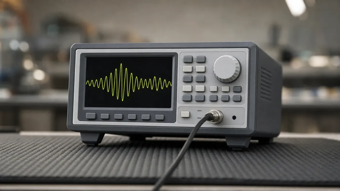
Set a bench generator to 2 V peak-to-peak, connect a coaxial lead to an oscilloscope, and there is a good chance the screen reads close to 4 V. Nothing is broken. The front panel states an intention; the device under test receives that intention after a converter has built it out of discrete samples, after an output path of finite bandwidth has rounded its edges, and after the instrument’s own source impedance has divided it against a load the instrument can only assume.
That gap between the requested signal and the delivered one is what a signal generator is actually chosen on. This guide is for engineers and technicians who already know what the instrument does and are now selecting one for a bench. It names no models and quotes no prices — model names date, and the reasoning behind a requirement does not. What it gives you instead is a way to turn the stimulus you actually need into a short ordered list of figures you can verify on any datasheet, and the reasoning that makes each figure defensible.
What the Device Under Test Actually Receives
A generator rarely works alone. It sits on one side of a device under test, and something that displays the response sits on the other; if you are still assembling that half of the bench, start with what an oscilloscope measures and how it works. The pairing only produces trustworthy conclusions if you know what went in — and what went in is not the number on the generator’s display.
Three transformations sit between the two. The waveform is built by a digital-to-analog converter that updates at a finite rate and holds its level between updates. It then passes through an output amplifier and analog filters of finite bandwidth, so the fastest transitions are rounded. Finally it meets the instrument’s own source impedance, in series with the output, which divides the voltage against whatever the load presents — a load the generator does not measure and can only be told about.
That reframes the datasheet usefully. Each specification line names one mechanism by which the delivered signal departs from the requested one:
- Bandwidth and sample rate — how fast the output is allowed to change, by two independent limits.
- Resolution — how finely the amplitude can be divided.
- Memory depth — how long a unique waveform runs before it repeats.
- Spurious free dynamic range, total harmonic distortion, signal-to-noise ratio, effective number of bits — further named departures from the requested signal.
- Phase noise, passband flatness, analog and digital filtering — the remaining named departures.
Choosing then becomes a bounded exercise rather than a comparison of feature lists: work out which of these mechanisms dominates for the stimulus you actually need, and bound that one first.
Start From the Signal You Need, Not the Waveform List
Most bad generator purchases are decided here, not in the specification table. An instrument that produces every shape you can name is still the wrong instrument if it cannot deliver that shape at the amplitude, into the load, and with the transition speed your DUT requires. So write the required stimulus down as five properties before opening a datasheet:
- The shape of the waveform.
- The fastest transition it has to contain.
- The amplitude at the load, including any DC offset.
- How the DUT input terminates —
50 Ω, high impedance, or something in between. - Whether that shape exists as one of the instrument’s standard functions, or has to be defined point by point.
The last property is the branch criterion, and it is cheap to settle. A function generator produces a set of standard periodic shapes — sine, square, triangle, pulse — and stores few points, because those shapes repeat. An arbitrary waveform generator reproduces a shape you define: a captured real-world signal, a modelled pulse, a modulation pattern. The dividing question is not how complicated the waveform looks but whether the wanted signal is one of the standard periodic ones. (On the bench, function generator is often used loosely for the whole class; on a datasheet it names this specific branch.) Comparing the two branches properly is its own subject; for a purchase, this single question usually picks the side.
Filling in the other four properties immediately tells you which specifications will bind. Suppose the DUT is a comparator input that must see a 1 V peak-to-peak square wave with a transition no slower than 10 ns, at the end of a short lead into a high-impedance pin. Three constraints are already fixed: the edge sets a bandwidth requirement, the high-impedance termination sets an amplitude correction you have to be able to declare on the instrument, and the shape is a standard function, so the branch question costs nothing. Nothing about waveform memory or fine frequency tuning matters for this stimulus, and no amount of either compensates for a restricted output path.
One property sends you out of this article altogether. If the required stimulus is a modulated carrier rather than a baseband waveform, the decision moves to the RF and vector generator family — a different class of instrument with a different specification vocabulary, and out of scope here. Everything below concerns the bench branch: function generators, arbitrary function generators and arbitrary waveform generators.
The Load the Instrument Assumes
Return to the surprise from the opening, because it is the single most consequential thing a datasheet’s amplitude specification depends on. A bench signal generator presents a nominal 50 Ω source impedance in series with its output, and that resistance forms a voltage divider with the load. Into a matched 50 Ω load, half the internally generated voltage drops across the internal resistance and half reaches the load. Into a high-impedance load — a 1 MΩ oscilloscope input, for instance — the divider is negligible and essentially the whole internal voltage appears at the connector. Same instrument, same setting, twice the amplitude.
Tektronix works the arithmetic through for its AFG3000 series. With the output set to 2 V peak-to-peak, the instrument generates 4 V internally. A 50 Ω load then receives (50/100) × 4 V = 2 V, exactly the set value. A 1,000 Ω load receives (1,000/1,050) × 4 V = 3.8095 V. A 1,000,000 Ω load receives (1,000,000/1,000,050) × 4 V = 3.9998 V. Note where the transition happens: by a kilohm the load is already behaving almost as an open circuit for this purpose, so “high impedance” is reached long before the megohms of an instrument input.
So what does the output load setting do? Not what its name suggests. It does not change the source impedance, which is fixed in hardware. It tells the instrument which load to assume, so that it can scale the internally generated voltage and make the displayed amplitude match what will appear at the load. On the AFG3000 series the setting is available per channel and accepts 50 Ω, a Load value anywhere from 0 to 10 kΩ, or High Z for anything above 10 kΩ; the generator then calculates the output voltage to apply for the load it has been told about.
This matters more than it should because most generators have no measurement function at all. You can set the amplitude; the instrument has no way of verifying that its true output matches that set value. Siglent’s own guidance is to check the waveform with an oscilloscope or DMM — while remembering that both usually present high-impedance inputs of 1 MΩ or greater, which is itself one side of the divider you are trying to characterise. An instrument whose termination setting you cannot declare is an instrument whose amplitude specification you cannot use.
When the Oscilloscope Is the Load
The case worth committing to memory is the one you meet daily: generator set to 50 Ω, load is an oscilloscope input at 1 MΩ or greater. The majority of the voltage drop is then across the external load, the set amplitude is roughly half the measured voltage, and the display under-reports what the DUT is getting by about a factor of two.
The fix is not automatically to change the setting. Terminating deliberately in 50 Ω — using the oscilloscope’s 50 Ω input setting, or an external feedthrough termination — is the configuration Tektronix identifies as giving the best system performance, and it is the right answer whenever edge fidelity matters, because the alternative invites very high frequency ringing on the fast transitions of a square wave. Working into a high impedance is the deliberate low-frequency choice: as much as double the output voltage, at frequencies where that ringing is not a concern. The four combinations behave as follows.
| Termination setting | Actual load | Amplitude at the load |
|---|---|---|
| 50 Ω | 50 Ω termination | Equals the display (2 V set gives 2 V delivered) |
| 50 Ω | High impedance (1 MΩ scope input) | About twice the displayed value |
| High Z | High impedance (1 MΩ scope input) | Equals the display |
| High Z | 50 Ω termination | About half the displayed value |
Bandwidth and Sample Rate Are Not One Specification
Two numbers on the front page of a generator datasheet are routinely quoted as though they were one. A 1 GS/s sample rate does not mean the instrument can put out 500 MHz of content, and it certainly does not mean it can hand you a 1 ns edge. They bound different things, and only one of them bounds edges.
Generator bandwidth is the frequency range over which output content is reproduced within 3 dB; above that figure, content is attenuated further. It is the same definition used on the acquisition side of the bench, developed at length in understanding oscilloscope bandwidth and how it is defined, so the space here is better spent on the consequence.
The consequence starts with where the limit comes from. National Instruments attributes a generator’s bandwidth to the output amplifier design and to filters in the analog output circuit — the analog path after the converter, not the converter’s update rate. Published instruments therefore place their analog output capability at a fraction of their sample rate:
- NI 5411 PXI module:
100 MS/s, sine output to43 MHz, square to25 MHz. - Tektronix AWG4000 in basic DDS mode:
2.5 GS/s, sine output to600 MHz. - Keysight 33600A TrueForm series: sampling to
1 GS/s, sinewaves to120 MHz.
Now the edge. Steepness lives in high-frequency content: a 10–90 % transition of duration tr has a knee frequency of 0.5/tr, so a 10 ns edge needs content out to 50 MHz, and a 2 ns edge out to 250 MHz. Read the other way, a band-limited path relates the two by bandwidth = k / rise time, with k between 0.35 and 0.45. Those relationships were established for oscilloscope front ends, and applying them to a generator’s output path is an engineering transfer rather than a vendor specification — but the band-limiting physics is the same, and the practical conclusion is firm: an instrument specified to 43 MHz will not deliver a 2 ns transition however fast its converter runs.
None of this makes sample rate irrelevant. It bounds the digital construction of the waveform, which must be updated at least twice as fast as the highest frequency it contains to be generated accurately. And at the top of the frequency range the two limits meet: the NI 5411 at its 43 MHz sine limit receives only about 2.3 converter updates per period, which is a constraint on shape in its own right.
How the Waveform Is Built
A converter does not draw curves. It holds a voltage until it is told to change. NI’s illustration of an ideal 20 MS/s converter generating a 1 MHz sine shows exactly that: a staircase of held levels, twenty per period, tracking the intended sine. The waveform your DUT sees begins life as that staircase, and the interesting question for a purchase is how many steps it gets and what happens to them afterwards.
The number of steps is simply the sample rate divided by the output frequency, and it collapses at the top of an instrument’s range. Twenty updates per period is comfortable. At their published sine limits, the three instruments above are working with about 8.3 updates per period (Keysight 33600A, 120 MHz on 1 GS/s), about 4.2 (Tektronix AWG4000 in DDS mode, 600 MHz on 2.5 GS/s), and about 2.3 (NI 5411, 43 MHz on 100 MS/s). The useful reading of a sample-rate figure is therefore not the number itself but the ratio it leaves you at your working frequency. Nyquist’s factor of two is a floor for generating a waveform at all, not a target; NI’s own guidance is that a rate many times the highest frequency present is what produces accurate waveforms, because a higher rate defines the shape more precisely.
What becomes of the staircase is the analog output path’s business. NI states that the filters in the analog output circuit, together with the output amplifier design, are what limit the source bandwidth — so those filters determine which of the frequency components the converter produced actually reach the connector. Reading that same filtering as the thing that smooths held levels into a continuous waveform is a reasonable working interpretation rather than a specification you can quote. What you can quote is that the output path is band-limited, and that its bandwidth is the figure printed on the datasheet.
On the arbitrary side, the construction works differently and the difference is worth understanding before you compare specifications. An arbitrary waveform generator converts stored samples continuously, point by point, one sample per cycle of a variable-frequency reference clock. Output frequency is set by that clock’s frequency, and the waveform shape stays constant as the clock changes, because every stored point is played at every frequency. That is the property to hold on to: on a true AWG, the shape you programmed is the shape that comes out, scaled in time.
Memory depth is how many samples the instrument can store for one waveform, and it sets how long a unique waveform runs before it repeats. Play time is memory depth divided by sample rate: 256 million samples at 100 MS/s gives 2.56 s, and the same memory emptied faster lasts proportionally less. This is generator memory — it holds the waveforms to be played out, plus the instructions for sequencing them — which is the mirror image of the acquisition memory covered in oscilloscope memory depth and what it buys you. The form of the trade-off is identical: depth buys time at a given rate, and rate spends it.
Frequency Resolution and What It Costs
Very fine frequency steps come from a different synthesis method. A direct digital synthesis generator — also known as an arbitrary function generator — holds waveform points in memory and reads them with a phase accumulator clocked at a fixed rate. Frequency is set by the phase increment: a larger increment skips memory locations and produces a higher frequency, a smaller one repeats locations for a lower one. Because the sampling clock never changes, frequency changes are essentially instantaneous, and the same mechanism supports quick waveform reconfiguration, digital modulation and frequency hopping.
Two consequences follow. At higher output frequencies not every stored point is used, which is why discontinuous or transient shapes — fast pulse rise and fall times, for example — are difficult to create accurately this way: samples representing the transient event may not be clocked out. And the tuning side of the datasheet is separate from the spectral purity side. DDS sources running at high clock rates typically tune more finely than AWG sources, which is why DDS blocks are often built into AWG designs; the figure that tells you what else is in the output is the spurious free dynamic range, the ratio between the fundamental and the largest spur from DC to half the sampling rate, usually in dBc. Component-level examples give the order of magnitude: the AD9850, on a 125 MHz clock with a 32-bit tuning word, achieves better than 50 dB, while the AD9914 pairs 190 pHz tuning resolution with wideband SFDR better than -50 dBc. Read SFDR in the same breath as frequency resolution.
Vertical Resolution: Where Amplitude Stops Being Continuous
Resolution is the number of bits in the output converter, and it decides the smallest amplitude step the instrument can produce: the peak-to-peak output range divided by 2^N.
Work it through. A 3-bit converter on a 0–10 V range divides that range into eight levels and cannot generate a voltage difference smaller than 1.25 V. A 16-bit converter on the same range has 65,536 levels and steps of about 153 µV. Resolution is a limiting factor on the accuracy of the generated waveform — more detail is present as the bit count rises. At small output ranges, the practical reading is that the step size, not the bandwidth, sets the amplitude fidelity available.
The step scales with the range, so the range setting is part of the resolution. NI’s PXIe-5433 has 16-bit resolution and can output a peak-to-peak range as small as 0.00564 V when maximum output attenuation is applied; the formula puts the step at that range at 0.00564 V / 65,536 ≈ 0.086 µV. NI’s own page prints 0.116 µV for this example, a figure that does not satisfy the formula it publishes alongside; the arithmetic is given here so you can run it against whatever ranges your candidate instrument offers rather than trusting a quoted step.
Bits are not the whole amplitude story. All analog electronics have harmonic distortion: generating a tone causes the electronics to resonate at integer multiples of it. Total harmonic distortion sums the power in each harmonic and divides by the power in the fundamental, and by the time THD approaches -30 dB the distortion is visible in the time-domain waveform. SINAD extends the accounting to noise — RMS signal amplitude against the RMS sum of all other spectral components, harmonics included, DC excluded — and equals the sum of SNR and THD. Where the DUT’s own nonlinearity is the quantity of interest, these are the figures that decide whether the stimulus is clean enough for the DUT to be blamed for what you see.
Channels
Multi-channel instruments are ordinary — the Tektronix AWG4000, for instance, has two channels, each capable of sine output to 600 MHz in basic DDS mode. The question is whether the second channel is a requirement or a convenience, and that turns on whether your test needs two signals with a defined relationship between them: a differential pair, a clock alongside a data stream, a signal and its reference.
One practical warning follows directly from the load discussion. Channel settings are independent: on the AFG3000 series the load impedance is set per channel. A two-channel instrument therefore carries two separate termination assumptions, and configuring one channel correctly says nothing about the other.
What the datasheet will actually give you on this point is the channel count and whether settings such as load impedance are independent per channel.
What a Datasheet Does Not Tell You
Two things the specification table never states change how the instrument behaves in daily use. The first is that the front-panel amplitude is a prediction. Most generators have no measurement function, so the displayed value is what the instrument expects to produce given the load it has been told to assume. Verification lives at the DUT end, with an oscilloscope or DMM — while remembering that those high-impedance inputs are themselves part of the circuit being measured.
The second is that headline figures are conditional and not necessarily simultaneous. Resolution step size depends on the selected output range. Bandwidth bounds the maximum output frequency regardless of converter rate. And one instrument can publish different figures per operating mode: the AWG4000 functions as both an AWG and a DDS, and in its basic DDS mode it is specified at 2.5 GS/s with 14-bit resolution and 16 kpoints of arbitrary waveform memory. Before comparing two candidates, confirm that the numbers you are comparing are stated under the same conditions and hold at the same time.
Then there is a category of properties that decides whether an instrument survives a real bench and which no generic guidance can answer for you: what happens to the output stage when it is connected to a powered DUT, how the output settles after an amplitude or range change, how the connectors hold up to daily reconnection, and how the remote-control interface fits your scripting workflow. These are rarely in the specification table. Put them to the vendor in writing, look for them in the user manual, or establish them on an evaluation unit. One related caveat is documented and worth carrying with you: an inadequately terminated line can ring on fast square-wave transitions, so the output configuration you adopt is part of the instrument’s practical behaviour, not a detail.
Turning This Into a Requirement Profile
The output of all this is not a model name. It is a short ordered list you can carry to any datasheet, built by mapping each property of your required stimulus onto the mechanism that bounds it.
- Amplitude at the load. Check the source impedance and confirm the instrument lets you declare the termination you will actually use. An amplitude specification you cannot tie to a stated load assumption cannot be used at all, which is why this comes first.
- Fastest required transition. Convert it to a frequency —
0.5/trfor a10–90 %edge — and require an output bandwidth above that figure. Not a sample rate. - Shape. If it is one of the standard periodic functions, the function-generator branch suffices. If it has to be defined point by point, you need the arbitrary branch, and with it a sample rate that leaves a comfortable number of updates per period at your top frequency and a memory depth that yields the play time you need.
- Amplitude fidelity. Turn your smallest meaningful amplitude step into a bit count against the range you will actually use, and if the DUT’s own nonlinearity is the measurement, read THD and SFDR as well.
- Frequency resolution. Only if you need very fine steps or fast hopping. Direct digital synthesis provides them, and SFDR is the figure to check alongside.
Then apply the rule that keeps a specification comparison from degenerating into a shopping list: identify which mechanism dominates for the stimulus you actually need, and bound that one properly before trading anything else away. Sources of both architectures exist because they are chosen for different performance capabilities, and an instrument that is generous everywhere except at your binding constraint is the wrong instrument at any price.
Frequently Asked Questions
Why does my oscilloscope show twice the amplitude I set on the generator?
Because the generator is almost certainly set to assume a 50 ohm load while the oscilloscope input presents 1 megohm or more. Most of the internally generated voltage then drops across the external load rather than across the generator's own 50 ohm source impedance, so the delivered amplitude is roughly double the displayed value.
What does the High-Z output setting actually change?
Only the arithmetic behind the displayed amplitude. The source impedance is fixed in hardware, and the setting simply tells the instrument which load to assume so that it can scale the internal voltage and make the display match what will appear at the load.
Does a 1 GS/s generator produce 500 MHz signals?
No. Sample rate bounds the digital construction of the waveform, while the analog output amplifier and filters set the bandwidth that decides what leaves the connector. The Keysight 33600A series samples to 1 GS/s but specifies sinewaves to 120 MHz.
How many bits of vertical resolution do I need?
Work from the smallest amplitude step your test requires: the step size is the peak-to-peak output range divided by 2 to the power of the bit count, so 16 bits across a 0 to 10 V range gives about 153 microvolts. Choosing the smallest range that fits your signal, with an offset, recovers resolution that a wider range would waste.
Can I trust the amplitude shown on the front panel?
Treat it as a prediction rather than a measurement, because most generators have no measurement function and cannot verify their own output. Confirm the amplitude at the device under test with an oscilloscope or DMM, keeping in mind that their high-impedance inputs are themselves part of the circuit.
Filed under
Related articles
Electronics18 min read
Function Generator vs Arbitrary Waveform Generator: What You Are Buying
Three names, two architectures: how DDS and point-by-point playback differ, what the labels hide, and how to read the architecture off a datasheet.
Electronics22 min read
How to Choose a Multimeter: A Specification-Led Buying Guide
Choose a multimeter by the errors it introduces: burden voltage, input loading, AC bandwidth, safety category and accuracy on the reading you actually take.
Electronics16 min read
How to Use a Thermal Camera: Getting Readings You Can Trust
A thermal camera always shows a number. Learn the checks — emissivity, reflected temperature, focus and spot size — that decide whether it is a measurement.
Electronics21 min read
FFT on Oscilloscopes: Principles, Setup, and Interpretation
How an oscilloscope's FFT function works, how sample rate, record length and window functions affect the result, and how to interpret an FFT spectrum in engineering work.