Oscilloscope Memory Depth Explained: Why It Matters
Learn what oscilloscope memory depth is, how it affects sample rate and acquisition time, and how to choose the right memory depth for accurate signal analysis.
By YDT EditorialUpdated 25 min read
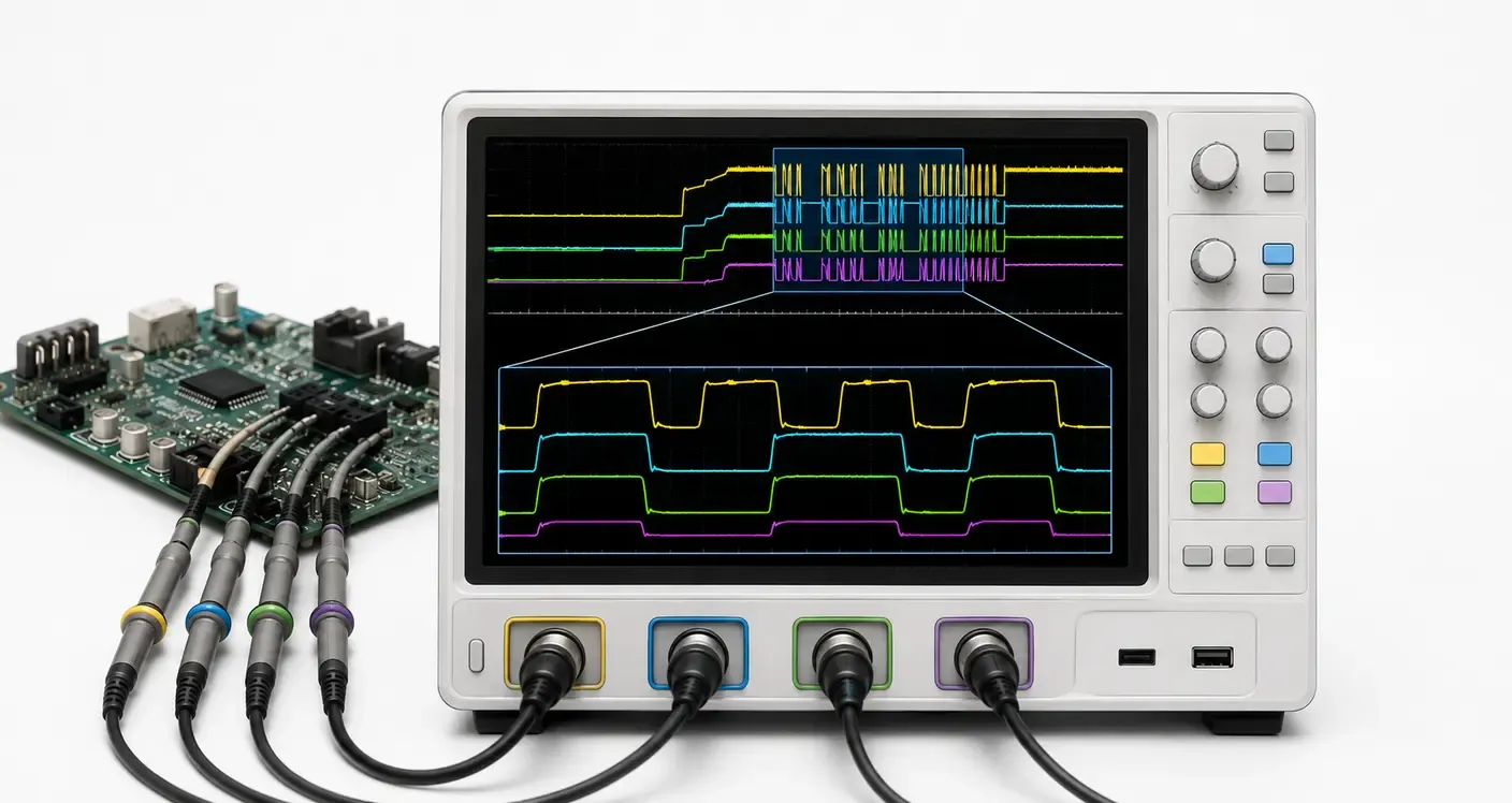
Most engineers meet memory depth by accident. You are chasing a glitch that appears somewhere during a start-up sequence, so you slow the timebase to see the whole sequence at once — and the glitch disappears. Nothing about the circuit changed. Nothing about the trigger changed. The waveform on screen still looks perfectly reasonable. What changed is that the oscilloscope quietly stopped sampling fast enough to see the event.
That is memory depth. It is the number of sample points an oscilloscope can store in a single acquisition, and it decides how long a window of time the instrument can capture before it has to start throwing detail away.
Bandwidth and sample rate describe how faithfully an oscilloscope can represent fast signal content. Memory depth describes how much of that content it can hold. An instrument with excellent bandwidth and a shallow acquisition buffer will show a fast edge beautifully, and will be unable to show what happened three milliseconds earlier.
Memory depth is one of the core specifications covered in our Test & Measurement: Complete Guide to Electronic Test Equipment resource, which places the full range of instruments and measurement techniques in context.
What Is Oscilloscope Memory Depth?
Definition
Memory depth is the size of the acquisition buffer an oscilloscope allocates to a single channel for a single capture, measured in sample points. Each point is one measurement of the input voltage taken at one instant by the analog-to-digital converter. Points are stored consecutively, so a completed record is simply a time-ordered list of voltage values separated by a fixed sample interval.
The distinction worth holding onto is that memory depth describes capacity, not speed. It says nothing about how quickly the samples were taken, only how many of them the instrument can keep. Sample rate is the shutter. Memory depth is the size of the film reel.
Why Memory Depth Is Measured in Points
Datasheets specify memory in points rather than bytes because a point maps directly onto time. Multiply the number of points by the sample interval and the result is the duration of the capture — the only quantity the engineer actually cares about at the bench.
Bytes do not behave this way. An 8-bit acquisition typically stores one byte per sample, while a 12-bit acquisition usually occupies two, so identical byte counts can represent very different record lengths. This is also why some instruments show reduced usable record length in high-resolution modes: the buffer is the same, but each sample costs more to store.
Expressing memory in points keeps the specification independent of vertical resolution, which is described separately by the ADC resolution of the instrument. The two parameters answer different questions: resolution governs how precisely each sample represents voltage, memory depth governs how many samples exist.
Record Length vs Acquisition Memory
These terms are used interchangeably in most product literature, but there is a distinction that explains a common frustration.
Acquisition memory is the physical capacity of the buffer — the maximum number of points the hardware can hold.
Record length is the number of points actually captured in a given acquisition. It depends on the timebase setting, the acquisition mode, the number of active channels and, on many instruments, a manual memory-depth selection with Auto and Manual options.
This last point trips people up regularly. An engineer buys an instrument specified at 100 Mpts, leaves the memory setting on Auto, and never observes anything close to that figure. Auto mode is usually tuned to keep the display responsive rather than to fill the buffer, and the full depth only appears once the setting is placed in Manual. The headline number on the datasheet is a best case: one channel active, memory forced to maximum, no acquisition mode restrictions.
How Oscilloscope Memory Depth Works
Knowing what memory depth is does not yet explain why it changes the measurement. That only becomes visible once the instrument runs out of it.
Memory Depth, Sample Rate and Acquisition Time
Return to the situation from the introduction, but this time watch what the instrument does.
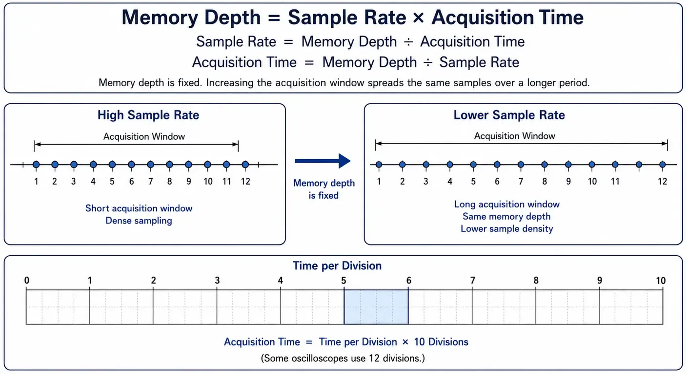
An oscilloscope specified at 1 GSa/s is set to 1 ms per division. With ten horizontal divisions, the displayed window is 10 ms wide. Filling that window at the full sample rate would require ten million points. If the instrument holds one million, it cannot do it.
Faced with this, the oscilloscope does not shorten the window. It reduces the sample rate until the record fits — in this case to 100 MSa/s. The display looks identical. The sample interval has grown by a factor of ten.
Most instruments show the current sample rate somewhere on screen, and turning the timebase knob while watching that readout is probably the single most useful five minutes an engineer can spend with a new oscilloscope. The number holds steady across the fast settings, then begins to fall, and the setting at which it starts falling is the practical boundary of the instrument’s memory. Everything slower than that point is a compromise.
This interaction is also why the oscilloscope time base setting has a direct effect on acquisition quality rather than only on what is displayed.
The Core Formula
Three parameters are locked together:
Memory depth = sample rate × acquisition time
The formula can be rearranged in whichever direction the question requires:
- Acquisition time = memory depth ÷ sample rate
- Sample rate = memory depth ÷ acquisition time
Acquisition time is derived from the timebase:
Acquisition time = time per division × number of horizontal divisions
Most oscilloscopes use ten horizontal divisions; some designs use twelve or more.
The useful mental model here is a budget. Memory depth is a fixed allowance of samples, and the timebase decides how thinly that allowance is spread across time. Widening the window does not buy more samples; it spends the same ones over a longer interval. Fix any two of the three parameters and the third is determined. There is no setting that escapes this.
Worked Examples
Example 1 — Establishing the window. An instrument with 1 Mpts of memory sampling at 1 GSa/s produces a 1 ms record. Across ten divisions that is 100 µs per division. Any attempt to view a slower event forces a sample rate reduction.
Example 2 — Working backwards from the requirement. A switching power supply soft-start sequence lasts approximately 200 ms, and the switching edges of interest justify at least 100 MSa/s. The requirement is 200 ms × 100 MSa/s = 20 Mpts. An instrument holding 10 Mpts will capture the sequence at 50 MSa/s, which corresponds to a 20 ns sample interval — too coarse to characterize the switching transitions.
Example 3 — Serial bus capture. Observing 50 ms of CAN traffic at 500 kbit/s while retaining enough resolution for reliable decoding at 25 MSa/s requires 1.25 Mpts. This is achievable on most current instruments, but only if the available memory is not being divided across four active channels.
Notice that in each case the calculation ran in the same direction: from the measurement to the requirement, never from the datasheet to the measurement. That is the habit worth forming. Memory depth is not a number to compare between instruments in the abstract — it is a number to check against a window you have already decided you need.
| Memory depth | Window at 1 GSa/s | Window at 100 MSa/s | Window at 10 MSa/s |
|---|---|---|---|
| 10 kpts | 10 µs | 100 µs | 1 ms |
| 100 kpts | 100 µs | 1 ms | 10 ms |
| 1 Mpts | 1 ms | 10 ms | 100 ms |
| 10 Mpts | 10 ms | 100 ms | 1 s |
| 100 Mpts | 100 ms | 1 s | 10 s |
| 1 Gpts | 1 s | 10 s | 100 s |
Why Memory Depth Matters
Almost every interesting fault lives at the junction of two timescales. Something slow goes wrong — a supply fails to come up, a bus locks, a motor stalls — and the cause is something fast that happened at one particular moment inside that slow event. Deep memory exists to let both timescales coexist in the same record.
Capturing Long-Duration Signals
A motor start-up, a communication handshake, a power sequencing routine and an inrush current event all unfold over tens or hundreds of milliseconds, yet the behavior that explains a fault often occupies nanoseconds. Capture only the fast part and you cannot see when it occurred relative to everything else. Capture only the slow part and you cannot see what it was.
Preserving High Sample Rates
The specified maximum sample rate of an oscilloscope is only available at fast timebase settings. As the timebase is slowed, the instrument sustains that rate only for as long as memory allows.
This leads to a useful way of reading a datasheet: memory depth is what makes the sample rate specification real. Two instruments quoting an identical 2 GSa/s can behave completely differently at 10 ms per division, and the one with more memory will still be sampling fast when the other has decimated by two orders of magnitude. The relationship is developed further in our guide to oscilloscope sample rate.
Detecting Rare Events
Intermittent faults are, by definition, unlikely to appear inside a short capture window. Extending the observed interval increases the probability that the event falls within a record, and deep memory extends that interval without sacrificing the resolution needed to identify what the event actually was — a genuine glitch, a coupling artifact, or a legitimate signal misinterpreted by downstream logic.
Where an intermittent event is separated by long idle periods, segmented memory is frequently a better answer than raw depth. Segmented acquisition stores only the intervals surrounding each trigger and discards the dead time between them, which uses the available buffer far more efficiently. An engineer capturing one hundred CAN frames arriving once per second gains nothing from storing the near-empty intervals in between.
Zooming Without Losing Detail
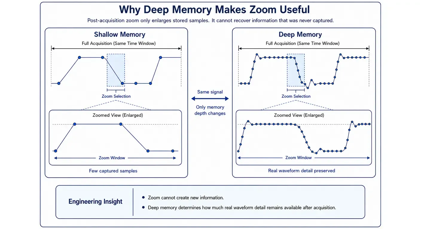
Post-acquisition zoom is a magnifying glass held over a photograph, not a second look at the scene. It displays samples that were already stored, and adds nothing. If the acquisition ran at a reduced sample rate because memory was exhausted, zooming reveals a sparse record and interpolated segments rather than the fine structure the operator expected.
This is the clearest practical argument for deep memory: it is what makes the zoom function honest. Capture a long window at full sample rate, then expand any region of it afterwards to inspect individual edges.
What Happens When Memory Depth Is Too Small?
Reduced Sample Rate
This is the primary and most consequential effect, and its defining characteristic is silence. The instrument decimates in order to preserve the requested window, because its priority is to give you the picture you asked for. Nothing on the display announces that the sample interval has changed by an order of magnitude, and the waveform continues to look entirely plausible.
The instrument protects the picture. It does not protect the physics.
Everything that follows in this section is a consequence of that single behavior.
Missed Glitches
A narrow pulse is captured only if a sample happens to fall inside it. Once the pulse is shorter than the sample interval, capture becomes a matter of probability rather than design — roughly the ratio of the pulse width to the sample interval on any given acquisition.
Put numbers on that and the consequence is obvious. A 20 ns glitch is comfortably resolved at 1 GSa/s, where the sample interval is 1 ns. At 10 MSa/s, with a 100 ns interval, roughly one acquisition in five will contain a sample inside the pulse, and even that sample may not land near its peak. The glitch has not gone away; the instrument has simply started rolling dice for it.
This interacts directly with oscilloscope triggering, and the interaction is easy to misread: a pulse-width trigger may correctly fire on an event that the acquisition record then represents with a single ambiguous sample. The trigger circuit is analog and sees the pulse. The record does not.
Aliasing Risks
Reducing the sample rate lowers the Nyquist frequency of the acquisition. Signal content above that limit does not disappear — it is folded back and displayed as lower-frequency content that was never present. The resulting waveform is stable, clean and wrong.
The trap is that the front end keeps its full bandwidth throughout. Nothing has been filtered out of the signal reaching the ADC, so the risk grows precisely at the moment memory forces the sample rate down. The mechanism is examined in detail in our article on aliasing.
Reduced Measurement Accuracy
Automatic measurements are computed from stored samples, so the achievable timing precision is bounded by the sample interval. Rise time, fall time, pulse width and period all depend on locating transitions within the record.
There is a recognizable symptom for this. When a rise time readout stops varying smoothly and instead steps between a few discrete values, the measurement has run out of samples across the edge, and the displayed number is reporting the sample interval more than it is reporting the signal.
A coarse record also shrinks the sample population available for statistical measurements such as jitter or histogram analysis, which is why those results grow noisier at slow timebases even when the signal has not changed.
Does More Memory Always Mean Better?
It is tempting to treat memory depth as a specification where the largest number wins. Spend an afternoon working with a fully loaded record and the trade-off becomes obvious: measurements take a moment to update, protocol decode lags behind the acquisition, and the instrument feels heavier under the hand. Deep memory is a tool with a cost, not a free upgrade.
Advantages of Deep Memory
- Long capture windows at full sample rate.
- Meaningful post-acquisition zoom across the entire record.
- Protocol decoding across many consecutive frames rather than isolated messages.
- Time correlation between slow control events and fast switching behavior.
- Larger sample populations for statistical and frequency-domain analysis.
Performance Trade-Offs
Every stored point must be transferred, processed, measured and rendered. Automatic measurements, FFT computation and protocol decoding across a 100 Mpts record take substantially longer than across 1 Mpts, and the difference is visible in front-panel responsiveness.
Transferring long records to a host computer over USB or LAN is slower still, which becomes a genuine workflow constraint in automated test, where the transfer rather than the acquisition sets the throughput of the sequence.
Deep memory also raises instrument cost, and on many mid-range and high-end oscilloscopes the largest memory configurations are licensed options rather than standard equipment.
Waveform Update Rate
Waveform update rate — the number of acquisitions processed per second — falls as record length grows, because each acquisition takes longer to capture and process. The interval between acquisitions is dead time, during which the instrument is blind.
The mental model is a strobe light in a dark room. A high update rate is a fast strobe: brief flashes, but many of them, so a moving object is likely to be lit at some point. A deep record is a long exposure: you see far more of what happens while the shutter is open, and nothing at all between exposures.
This creates a genuine tension, because there are only two ways to find a rare event — look for longer, or look more often — and memory depth improves one at the expense of the other. Modern instruments mitigate the conflict with hardware acquisition engines and segmented memory, but the trade-off does not disappear.
Shared Memory Between Channels
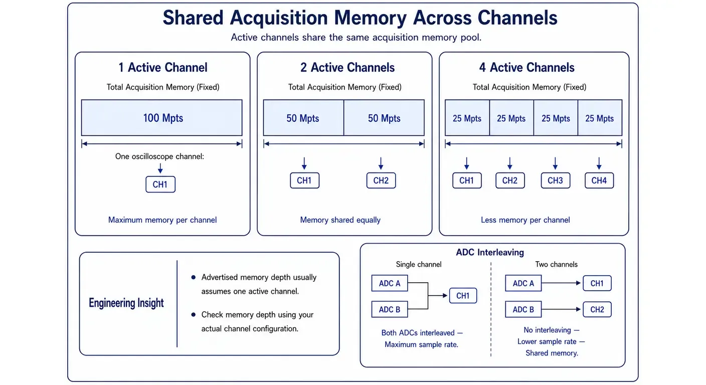
On many oscilloscopes the acquisition memory is a pool divided among active channels. Enabling a second channel halves the depth available to each; enabling four may quarter it. A separate but related architecture interleaves two ADCs to serve one channel at double the sample rate, so activating the paired channel reduces both sample rate and per-channel memory simultaneously.
The result is that a headline figure of, for example, 100 Mpts may correspond to 25 Mpts per channel in four-channel operation. This is normal engineering practice rather than a defect, but it has a practical implication worth internalizing: the configuration you will actually work in is usually the worst case.
Embedded debugging means four channels. Power electronics means at least two, often three. Evaluate the specification in that configuration, not in the single-channel one the datasheet leads with. Our guide to oscilloscope specifications covers how these conditional figures are usually presented.
Memory Depth vs Sample Rate
Key Differences
Sample rate is how finely the instrument slices time. Memory depth is how many slices it can carry away.
| Parameter | What it defines | Unit | Limits |
|---|---|---|---|
| Sample rate | How often the input is measured | samples per second | Time resolution, highest frequency that can be represented |
| Memory depth | How many measurements are retained | points | Duration of the capture at a given sample rate |
Sample rate governs detail. Memory depth governs duration. Neither specification is meaningful in isolation, and an instrument advertised on one of them alone should invite the question of what the other is doing.
How They Work Together
Raising the sample rate improves resolution but consumes memory faster. Increasing memory extends the window but does not improve resolution. An instrument is well balanced when it can sustain the sample rate its bandwidth justifies across the timebase settings its intended applications require — which is a more demanding test than either number passes on its own.
Practical Engineering Examples
High sample rate, shallow memory. 2 GSa/s with 10 kpts produces a 5 µs record. Excellent for characterizing a single fast edge. Useless for observing a complete serial frame.
Modest sample rate, deep memory. 100 MSa/s with 100 Mpts produces a 1 s record with a 10 ns sample interval. Excellent for observing a long control sequence. Insufficient for measuring nanosecond transitions within it.
Balanced configuration. 1 GSa/s with 50 Mpts produces a 50 ms record at a 1 ns sample interval — long enough for most embedded and power sequencing work while retaining edge detail throughout.
Memory Depth vs Bandwidth
Sample rate and memory depth are both digital specifications, and they compete for the same resource. Bandwidth belongs to a different part of the instrument entirely, which is why comparing it with memory depth requires a different way of thinking.
Different Specifications, Different Purposes
Bandwidth is an analog property of the front end, defined by the frequency at which the displayed amplitude has fallen by 3 dB. It determines what signal content reaches the ADC at all. Memory depth is a digital property of the acquisition system, applying only to samples that have already been converted.
Order matters here, and it is worth picturing the acquisition path as a one-way chain: probe, front end, ADC, memory. Each stage can only work with what the previous stage handed it. Content attenuated by the front end is not present in the digitized data, and no amount of memory can recover it. Conversely, bandwidth cannot extend an acquisition window by a single microsecond.
Why Both Matter
A complete acquisition path requires adequate bandwidth to admit the signal, an adequate sample rate to represent it, and adequate memory to retain it for the required duration. A shortfall anywhere in that chain limits the result regardless of the other two — and, awkwardly, the display gives no indication of which link failed.
The probe belongs in the same chain, and in practice it is often the weakest link, since probe bandwidth and ground lead inductance frequently limit the measurement before the instrument does. That subject is covered in our oscilloscope probe guide and alongside it in oscilloscope bandwidth explained.
Choosing the Right Memory Depth
The following table gives general reference ranges. Actual figures vary considerably between manufacturers, model generations and option levels, and should always be confirmed against the datasheet for the specific configuration under consideration.
| Instrument class | Commonly encountered maximum memory depth |
|---|---|
| Entry-level and educational bench oscilloscopes | Tens of kpts to approximately 25 Mpts |
| Mainstream four-channel bench oscilloscopes | Approximately 10 Mpts to 200 Mpts |
| Mid-range and high-performance bench instruments | Approximately 100 Mpts to 1 Gpts, frequently as a licensed option |
| High-end performance oscilloscopes | 1 Gpts and above per channel |
| PC-based and USB oscilloscopes | Wide range, constrained by instrument buffer and host transfer rate |
Embedded Systems
The typical embedded session has four probes attached — clock, data, chip select and an enable or interrupt line — and the question being asked is almost always about ordering: did this line assert before that one, and how long after reset. That question requires all four records to exist simultaneously over a window of a few milliseconds to tens of milliseconds, at a sample rate that still resolves logic edges.
Ten to fifty megapoints of usable per-channel depth is comfortable for this work. One megapoint becomes restrictive quickly once four channels are enabled, and the first symptom is usually protocol decode: the decoder stops producing frames at slower timebases because the sample rate has fallen below what it needs to resolve bit boundaries reliably.
Power Electronics
Switching converters are the clearest case of two timescales in one measurement. Soft-start behavior, load-step response and several cycles of a 50 Hz or 60 Hz line waveform all occupy 100 ms or more, while SiC and GaN switching edges justify sample rates in the hundreds of megasamples per second and gate-loop ringing sits higher still.
A window of 100 ms at 250 MSa/s corresponds to 25 Mpts, which sets a realistic lower bound. Anything less forces a choice between seeing the sequence and seeing the switching, and the fault usually lives in the relationship between the two.
Automotive Diagnostics
Automotive events are long by any bench standard. Cranking, injector sequences, sensor sweeps and network arbitration extend from hundreds of milliseconds to several seconds, while the underlying CAN, CAN FD and LIN traffic still requires adequate sampling to decode.
Depths in the tens to hundreds of megapoints are useful here, but segmented memory earns its keep more than raw depth: intermittent faults that appear once during a road test are exactly the case the feature was designed for.
Serial Communication Debugging
The requirement follows directly from the number of frames to be observed, which makes this the easiest case to size. Estimate the total duration of the traffic of interest, multiply by a sample rate providing several samples per bit period, and the result is the memory required.
One hundred CAN frames at 500 kbit/s occupy roughly 25 ms; captured at 50 MSa/s, that is 1.25 Mpts. Extending the observation to several hundred frames scales the requirement into the tens of megapoints. A slower bus does not automatically reduce the figure either, since the longer frame duration largely offsets the lower sample rate it needs.
Long-Duration Captures
Beyond a few seconds, raw memory depth becomes an inefficient solution and the right move is usually to change technique rather than to buy a bigger buffer. In order of preference: segmented memory, deliberate reduction of the sample rate where the signal content genuinely permits it, and — where only slow behavior matters — a data acquisition system or datalogger, which is designed for continuous recording rather than triggered capture.
| Application | Typical window | Sample rate needed | Approximate memory |
|---|---|---|---|
| Audio and low-frequency analog | 100 ms | 1 MSa/s | 100 kpts |
| General embedded debugging | 10 ms | 250 MSa/s | 2.5 Mpts |
| Serial bus decoding | 50–500 ms | 25–50 MSa/s | 1.25–25 Mpts |
| Switching power supply start-up | 200 ms | 100–250 MSa/s | 20–50 Mpts |
| Motor drive and inverter analysis | 1 s | 10–50 MSa/s | 10–50 Mpts |
| High-speed digital signal integrity | 1 ms | 5–20 GSa/s | 5–20 Mpts |
Read across the table and a pattern emerges: the demanding cases are rarely the fastest signals. They are the ones where a long window and a fine sample interval are required at the same time.
Common Misconceptions
“The oscilloscope always samples at its maximum rate.” It samples at the highest rate the available memory permits for the selected timebase. At slow timebases, actual sample rates are frequently one or two orders of magnitude below the specified maximum. The on-screen sample rate readout is the fastest way to confirm what is really happening.
“Deep memory compensates for insufficient bandwidth.” It does not. Memory stores what the front end and ADC produced. Attenuated content is absent from the record before memory becomes relevant.
“More memory always improves the measurement.” Deep records reduce waveform update rate and slow processing. For short, fast, repetitive signals, a shallow record at a high update rate is often the better instrument setting.
“Memory depth improves vertical accuracy.” Vertical accuracy is governed by ADC resolution, front-end noise and gain accuracy. Memory depth affects the time axis only.
“Zoom reveals more detail.” Zoom expands stored samples. If the record was acquired at a reduced sample rate, no additional detail exists to reveal.
“The number displayed equals the number stored.” A display is typically around a thousand columns wide, so rendering a 100 Mpts record necessarily decimates it. The full record remains available for measurement, zoom and decoding — which is why an on-screen waveform can look unremarkable while a measurement computed from the same acquisition reports something the eye never saw.
Memory depth rewards being treated as one term in a fixed equation rather than as a competitive specification. Establish the window an application requires, establish the sample rate its fastest content requires, multiply, and compare the result against the depth available in the channel configuration you will actually use. Engineers who form that habit stop being surprised by their instruments, because they already know where the sample rate is going to fall before they reach for the timebase knob. That calculation, considered alongside bandwidth, sample rate and probing, is what makes a specification comparison meaningful — a process set out in full in our guide to choosing an oscilloscope.
Frequently Asked Questions
What is oscilloscope memory depth?
It is the number of sample points the oscilloscope can store in one acquisition on one channel, quoted in kpts, Mpts or Gpts. Together with the sample rate it sets how much time you can capture, since memory depth equals sample rate multiplied by acquisition time. Think of sample rate as the shutter speed and memory depth as the length of the film.
Is 1 Mpts enough?
It depends on the window you need. One megapoint at 1 GSa/s gives you a 1 ms record, which is fine for repetitive digital and analog signals but tight for serial bus decoding, power supply start-up or any four-channel embedded work. For those, usable depth in the tens of megapoints is a more realistic starting point.
Is memory depth the same as record length?
In most datasheets, yes — the terms are used interchangeably. The distinction that matters in practice is that acquisition memory is the maximum the hardware can hold, while record length is what you actually captured, which depends on the timebase, the acquisition mode, how many channels are active and whether the memory setting is on Auto or Manual.
Does enabling more channels reduce memory depth?
On many instruments it does. Where the memory is a shared pool, each additional channel divides what is left. Some architectures also interleave converters, so turning on the paired channel costs you sample rate and memory at the same time. The datasheet usually quotes single-channel and all-channel figures separately, often with the second one in a footnote.
Can memory depth be upgraded?
Sometimes. Several mid-range and high-end instruments ship with the hardware already installed and unlock the extra depth through a software license, which can normally be bought later. Entry-level instruments generally have a fixed buffer with no upgrade path, so if you expect the requirement to grow, check this before you order rather than afterward.
How much memory do I need?
Work backwards from the measurement rather than forwards from the datasheet. Take the duration of the event you need to see, multiply by the sample rate required to resolve its fastest content, and that is your figure. Then check that the number is available with all the channels you intend to use switched on, not just one.
Related articles
Electronics18 min read
Function Generator vs Arbitrary Waveform Generator: What You Are Buying
Three names, two architectures: how DDS and point-by-point playback differ, what the labels hide, and how to read the architecture off a datasheet.
Electronics23 min read
How to Choose a Signal Generator: Getting the Signal You Asked For
How to turn a required stimulus into datasheet requirements: the load the instrument assumes, bandwidth against sample rate, reconstruction and vertical resolution.
Electronics22 min read
How to Choose a Multimeter: A Specification-Led Buying Guide
Choose a multimeter by the errors it introduces: burden voltage, input loading, AC bandwidth, safety category and accuracy on the reading you actually take.
Electronics16 min read
How to Use a Thermal Camera: Getting Readings You Can Trust
A thermal camera always shows a number. Learn the checks — emissivity, reflected temperature, focus and spot size — that decide whether it is a measurement.