What Is an Oscilloscope? How It Works, What It Measures & Common Uses
Learn what an oscilloscope is, how it works, what it measures, and when to use one. Understand waveforms, bandwidth, sampling, probes and triggering in this engineering guide.
By YDT EditorialUpdated 23 min read
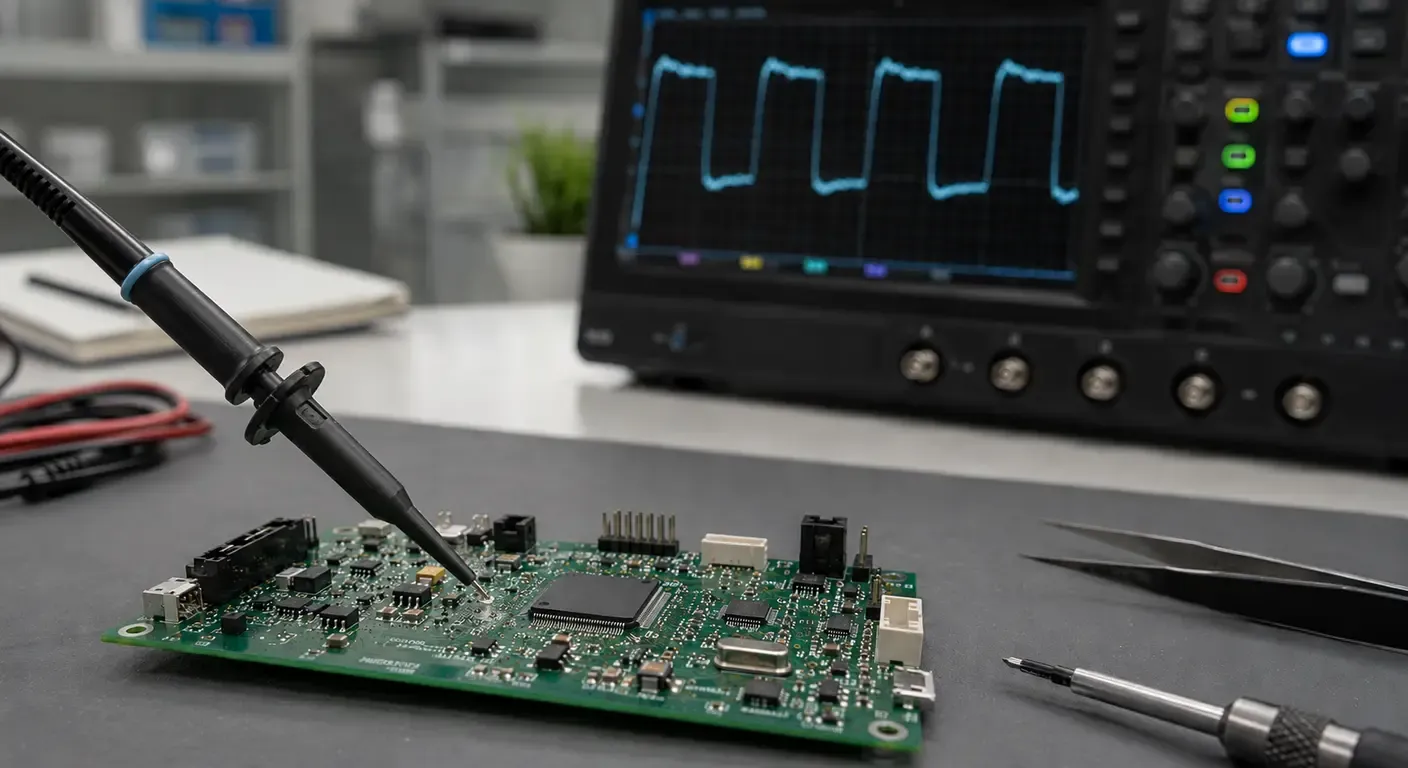
An oscilloscope is a test instrument that measures voltage as a function of time and displays the result as a waveform. Voltage occupies the vertical axis, time the horizontal axis, and the trace drawn between them shows the signal itself: its amplitude, its period, the speed of its transitions and any disturbance superimposed on it. Where a multimeter reports a single averaged value, an oscilloscope reproduces the behavior that produced that value. Engineers rely on the instrument for exactly that reason: most electrical behavior only becomes meaningful once it is observed over time rather than reduced to a single reading.
That distinction defines the instrument’s role on the bench. Almost every electronic circuit works with signals that change over time: a clock line toggling millions of times per second, a switching regulator chopping current, a sensor output drifting under load. A multimeter reduces that activity to a number. An oscilloscope shows the activity itself.
This is why the oscilloscope remains the central instrument in electronic design, debugging and maintenance. It turns invisible electrical behavior into a measurable, comparable picture. This guide explains what an oscilloscope measures, how it acquires and displays a signal, which types are available, how a basic measurement is set up, and when the instrument is genuinely necessary rather than simply convenient.
Central as it is, the oscilloscope answers only one kind of question. Our complete Test & Measurement guide sets out where it sits among multimeters, signal sources, spectrum analyzers and the rest of the bench.
What Is an Oscilloscope?
The Role of an Oscilloscope
The oscilloscope’s role in an engineering workflow is observational. It sits between the circuit and the engineer as a recording instrument, resolving electrical activity in both amplitude and time so that measured behavior can be compared against what the design intended.
The instrument does not interpret the circuit for you. It reproduces, as faithfully as its bandwidth and sampling capability allow, the voltage present at the probe tip relative to a reference point. Everything an engineer concludes from an oscilloscope, from a failing clock edge to excessive supply ripple, comes from interpreting that trace.
Why Engineers Use Oscilloscopes
Most difficult electronic faults are behavioral rather than static. A supply rail may measure a correct 3.3 V on a multimeter while carrying enough switching noise to reset a microcontroller. A serial line may look healthy until one edge arrives late. A motor drive may operate correctly at low load and oscillate at high load.
An oscilloscope makes these behaviors observable. It shows shape, timing, transient events and the relationship between two or more signals captured simultaneously, which is the information needed to explain why a circuit misbehaves rather than simply confirming that it does.
What Makes It Different from Other Test Instruments
Each instrument on a bench answers a different question. A digital multimeter answers what the value is, with high accuracy but no view of change over time. A logic analyzer answers what the digital state is, across many channels, but discards analog detail such as ringing or slow edges. A spectrum analyzer answers which frequencies are present, working in the frequency domain rather than the time domain.
The oscilloscope answers what the signal actually looks like. It offers fewer channels than a logic analyzer and lower absolute accuracy than a good multimeter, but it is the only common instrument that shows the real shape of a signal as it evolves.
What Does an Oscilloscope Measure?
Fundamentally, an oscilloscope measures one thing: voltage against time. Every other quantity listed below is derived from that pair of axes, either by the operator reading the graticule or by the instrument’s automatic measurement functions.
Voltage
The vertical axis represents instantaneous voltage at the probe tip, measured relative to the probe ground reference. Vertical sensitivity is set in volts per division, and the input can usually be DC coupled to show the full signal including its DC offset, or AC coupled to block the DC component and expand a small ripple riding on a large rail.
Time
The horizontal axis represents time, set in seconds per division. This is what allows periods, pulse widths, propagation delays and the interval between two events on different channels to be measured directly rather than inferred.
Waveforms
The shape of a trace carries most of the diagnostic information. Sine waves, square waves, triangular ramps, PWM pulse trains and exponential capacitor charging curves are all immediately recognizable, and deviations from the expected shape, such as flattened peaks, sagging plateaus or superimposed oscillation, point directly at the underlying fault.
Frequency
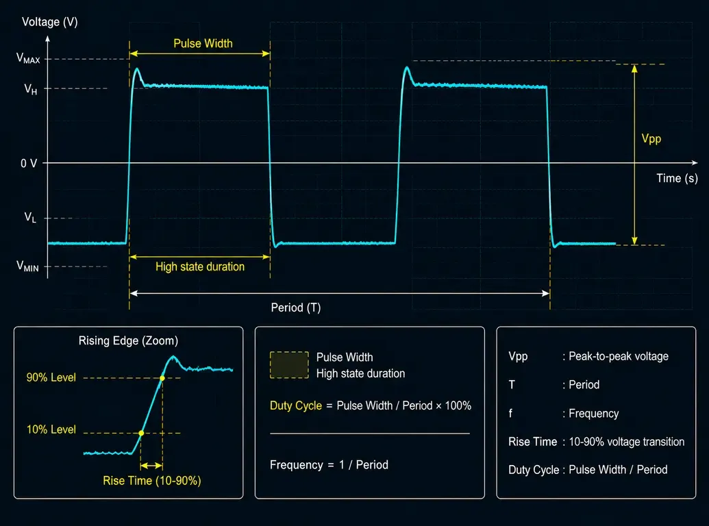
Frequency is derived from the period of a repetitive waveform, since frequency equals one divided by the period. Most digital oscilloscopes calculate this automatically. Accuracy depends on having enough samples per cycle and on the instrument’s bandwidth being comfortably above the signal frequency.
Signal Amplitude
An oscilloscope reads peak-to-peak amplitude directly from the screen, along with maximum, minimum and, on most digital models, calculated RMS values. This distinction matters: a multimeter typically reports an RMS value, while a designer checking whether a signal exceeds a logic threshold or an absolute maximum rating needs the peak.
Rise Time
Rise time is conventionally measured between the 10% and 90% points of a transition, and it characterizes how quickly a circuit can switch. In digital and power switching work it is often more informative than frequency, because it determines both timing margin and the high-frequency content the circuit generates.
It is also the measurement most affected by the instrument itself. The oscilloscope’s own rise time combines with the signal’s rise time, and the two add approximately in quadrature, so a scope whose rise time is comparable to the signal under test will report edges that are slower than reality.
For instruments with a Gaussian frequency response, scope rise time is commonly estimated as 0.35 divided by the bandwidth, a rule of thumb that becomes less reliable for high-bandwidth models with flatter responses. Where accurate edge measurement matters, the relationship between oscilloscope bandwidth and rise time should be checked against the manufacturer’s stated response.
Duty Cycle
Duty cycle is the ratio of the active portion of a pulse to the full period, expressed as a percentage. It is central to PWM applications such as motor speed control, LED dimming and switch-mode power conversion, where the duty cycle directly sets the delivered energy.
Noise and Signal Integrity
Ripple on a supply rail, ringing after a fast edge, crosstalk from an adjacent trace, ground bounce and reflections on an unterminated line all appear as time-domain artifacts. These are invisible to an averaging instrument, and they are frequently the root cause of intermittent behavior in otherwise correct designs.
How Does an Oscilloscope Work?
Signal Acquisition
The signal path begins at the probe and enters the input stage, where an attenuator and amplifier scale it to a level the digitizer can handle. General-purpose inputs typically present a high impedance of 1 MΩ in parallel with a small input capacitance, which suits most low and medium frequency work. Higher-bandwidth instruments often provide a 50 Ω input intended for terminated transmission-line measurements.
Sampling
In a digital oscilloscope, the conditioned signal is converted by an analog-to-digital converter, or ADC, into a stream of numeric samples. Everything displayed afterwards is a reconstruction of those samples.
Sample rate determines how finely the waveform is described in time. Sampling theory requires at least twice the highest signal frequency, but practical waveform reconstruction usually calls for several times that. Insufficient sampling produces aliasing, where a fast signal is displayed as a slower one that never existed, and the resulting trace can look entirely plausible.
Memory depth determines how long the instrument can record at a given sample rate. Once memory is exhausted, a longer time base is only possible by reducing the sample rate, which is why memory depth and sample rate must be considered together rather than in isolation.
Vertical resolution is set by the ADC. Eight bits remains typical for general-purpose models, with higher-resolution instruments available where small signals must be resolved on top of large ones.
Displaying Waveforms
Samples held in acquisition memory are processed and drawn on the display, usually with interpolation between sample points so that the trace appears continuous. The rate at which the instrument repeats this cycle, known as the waveform update rate, determines how likely it is to catch a rare glitch, since events occurring during processing are simply not captured.
Triggering
Without triggering, successive acquisitions would start at arbitrary points and a repetitive signal would appear as an unstable blur. The trigger defines the condition that starts a capture, most commonly a rising or falling edge crossing a chosen voltage level.
Because a digital oscilloscope samples continuously into memory, it can also display what happened before the trigger point, which is often the most useful part of a fault capture. Advanced trigger types respond to pulse width, dropped edges, runt pulses or decoded serial patterns, and oscilloscope triggering is frequently the difference between observing an intermittent fault and never seeing it at all. Our dedicated guide to oscilloscope triggering covers trigger types and setup in depth.
Understanding the Screen Grid
The display is divided by a graticule, commonly eight divisions vertically and ten horizontally. Multiplying divisions by the volts-per-division and seconds-per-division settings gives amplitude and timing directly, which is why experienced users still read the grid even when automatic measurements are available: it provides an immediate sanity check on whether an automatic value is plausible.
Main Components of an Oscilloscope
Display
The screen presents the waveform, the graticule, channel scaling information, trigger settings and automatic measurements. On modern instruments it also hosts the menu system, so display size and clarity have a direct effect on how quickly the instrument can be operated.
Input Channels
Two-channel and four-channel models are the most common. Multiple oscilloscope channels allow signals to be compared in time, such as a control input against the resulting output. On almost all mains-powered bench instruments the channel grounds are connected together and referenced to protective earth, a constraint that shapes how the instrument may be safely connected.
Vertical Controls
Vertical controls set volts per division, vertical position, input coupling, optional bandwidth limiting to reduce displayed noise, and the probe attenuation factor. The attenuation setting must match the probe in use, otherwise every amplitude reading will be wrong by that factor.
Horizontal Controls
Horizontal controls set the time base in seconds per division and the horizontal position, which determines how much pre-trigger and post-trigger data is shown. A zoom or delayed time base allows a short region of a long capture to be expanded without a new acquisition.
Trigger Controls
These select the trigger source, level, slope and type, together with the trigger mode. Auto mode free-runs when no trigger occurs and is useful when hunting for an unknown signal; normal mode updates only on a valid trigger; single mode arms once and is the correct choice for capturing a one-off event.
Oscilloscope Probes
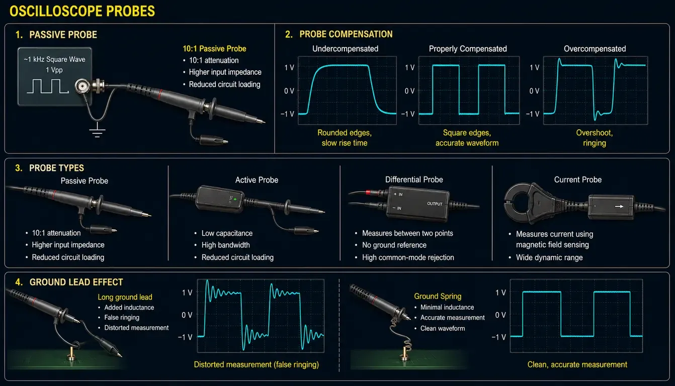
The probe is part of the measurement system, not an accessory. A 10:1 passive probe attenuates the signal tenfold, which raises the effective input impedance and reduces capacitive loading on the circuit under test.
Passive probes with adjustable compensation must be trimmed against the instrument’s calibration output. An uncompensated probe will display false overshoot or rounding on square waves, and the error follows every measurement made with it. Our oscilloscope probe guide covers probe types, attenuation, loading and compensation in depth.
Active probes reduce loading further at high frequency, differential probes measure between two points without a ground connection, and current probes sense magnetic field rather than voltage.
A long ground lead adds inductance and is a common cause of apparent ringing that exists only in the measurement, so the ground connection should be kept as short as practical when observing fast edges.
Common Applications of Oscilloscopes
Electronics Design
During prototype bring-up, an oscilloscope verifies that supply rails start cleanly, that clocks and reference signals meet their expected shape and frequency, and that analog stages behave as simulated. It is usually the first instrument reached for when measured behavior departs from the design intent.
PCB Debugging
On a populated PCB, layout problems appear as signal integrity problems: overshoot on fast edges, coupling between adjacent traces, and timing margins that shrink under load. Observing these directly is far more efficient than deducing them from functional symptoms alone.
Power Electronics
Switching converters, gate drivers and motor drives are inherently time-domain devices. Engineers use oscilloscopes to inspect switching node transitions, gate drive quality, dead time, output ripple and current waveforms, generally with differential and current probes suited to the voltage levels involved.
Automotive Diagnostics
Vehicle systems generate characteristic waveforms: crankshaft and camshaft sensor outputs, injector and ignition pulses, and communication traffic on buses such as CAN. Comparing a captured waveform against a known-good reference frequently isolates an intermittent fault that fault codes alone cannot explain.
Industrial Maintenance
In plant environments, oscilloscopes are used to examine variable frequency drive outputs, encoder signals, sensor lines and fieldbus communication, and to capture intermittent disturbances that appear only under specific machine conditions. Portability and adequate isolation usually matter more than maximum bandwidth here.
Research and Education
In laboratories and teaching environments, the oscilloscope provides a direct visual link between theory and measured behavior. Watching a capacitor charge, a filter attenuate or an amplifier clip makes abstract circuit theory concrete in a way that numerical readings do not.
Types of Oscilloscopes
Analog Oscilloscopes
Analog instruments deflect an electron beam across a cathode ray tube in direct proportion to the input signal. They display continuously and with no processing delay, which some users still value, but they cannot store a waveform, offer no automatic measurements, and are limited to repetitive signals. They have largely been replaced by digital models.
Digital Storage Oscilloscopes (DSOs)
The digital storage oscilloscope digitizes the input and holds it in memory, which makes single-shot capture, automatic measurement, cursor readout, saving and post-capture analysis possible. This is the standard instrument on modern benches and the default assumption in most current documentation.
Mixed Signal Oscilloscopes (MSOs)
A mixed signal oscilloscope adds a group of digital-only input channels alongside its analog channels. This suits embedded systems work, where an analog view of one line must be correlated with the logic state of several others, and where built-in decoding of serial buses turns raw edges into readable protocol data.
Handheld Oscilloscopes
Handheld models are battery powered and built for field use. Many provide isolated input channels, which is a significant safety advantage when measuring in equipment that is not earth-referenced. Bandwidth, memory depth and display size are generally more modest than on a comparable bench instrument.
USB Oscilloscopes
USB or PC-based instruments move the display and user interface onto a computer, keeping only the acquisition hardware in an external module. This lowers cost and can allow generous memory depth, at the expense of front-panel controls and of depending on a host computer, which some users find slower to operate for quick measurements.
| Oscilloscope type | Best suited for | Main strength |
|---|---|---|
| Analog | Legacy equipment and teaching benches | Continuous, unprocessed display |
| Digital storage (DSO) | General design, debugging and repair | Capture, storage and automatic measurement |
| Mixed signal (MSO) | Embedded and bus-level development | Correlated analog and logic channels |
| Handheld | Field service and on-site diagnostics | Portability and input isolation |
| USB / PC-based | Cost-sensitive and automated setups | Acquisition capability per unit cost |
Oscilloscope vs Multimeter
What a Multimeter Can Measure
A digital multimeter measures DC and AC voltage, current, resistance and continuity, and commonly capacitance, diode drop, temperature and frequency. Its strength is accuracy on steady quantities: a mid-range meter resolves values far more precisely than the vertical accuracy of a typical oscilloscope, and it is faster to use for a simple check.
Its limitation is that it reports a single number derived over a measurement interval. Anything shorter than that interval, and anything about the shape of the signal, is lost.
When an Oscilloscope Is Necessary
An oscilloscope becomes necessary as soon as the question involves time: whether an edge is fast enough, whether two events are correctly sequenced, whether a rail is clean under load, whether a glitch occurs and how often. It is also necessary whenever a waveform is non-sinusoidal, since an AC multimeter reading on a distorted or pulsed signal can be misleading unless the meter is true RMS and rated for that content.
Using Both Instruments Together
The two instruments are complementary rather than competing, and most troubleshooting uses them in sequence: the multimeter to confirm that levels are broadly correct, the oscilloscope to explain why correct levels are still producing incorrect behavior.
| Measurement need | Digital multimeter | Oscilloscope |
|---|---|---|
| Precise steady DC voltage | Preferred | Adequate |
| Resistance and continuity | Preferred | Not available |
| Supply ripple and noise | Not visible | Preferred |
| Timing between two signals | Not possible | Preferred |
| Rise time and edge quality | Not possible | Preferred |
| Intermittent glitch capture | Not possible | Preferred |
| Current measurement | Direct, with meter in circuit | Requires current probe or shunt |
How to Use an Oscilloscope (Basic Workflow)
Connecting the Probe
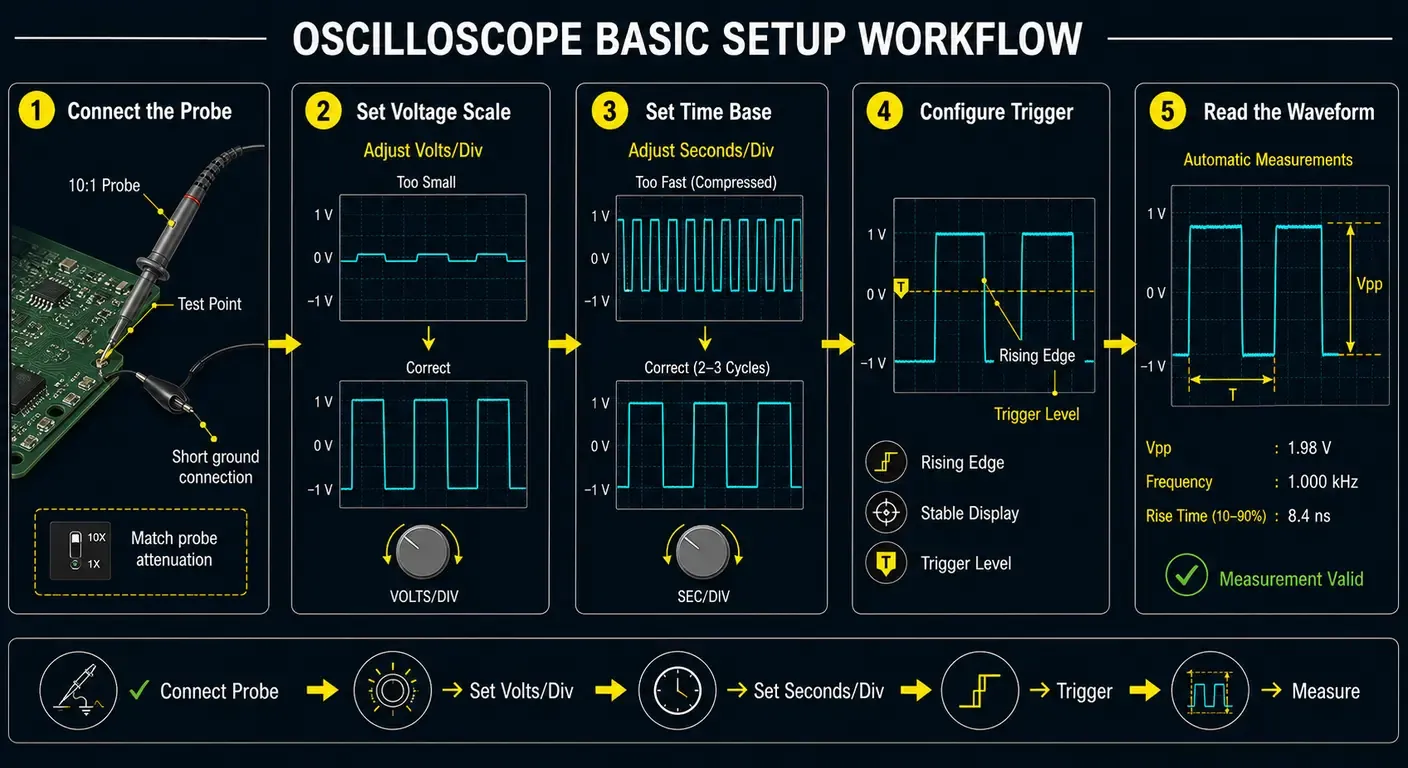
Set the probe to its intended attenuation and confirm that the channel menu is set to match. Compensate a passive probe against the instrument’s calibration output before precise work. Attach the ground clip to a solid circuit reference as close to the test point as practical, then touch the tip to the node of interest.
Choosing Voltage Scale
Begin with a coarse volts-per-division setting so that an unexpectedly large signal stays on screen, then reduce the scale until the waveform occupies most of the vertical graticule. Select DC coupling to see the true level, or AC coupling to expand a small variation on a large offset.
Setting the Time Base
Adjust seconds per division until a few complete cycles are visible. Two or three cycles is usually the most readable compromise: enough to confirm the signal is stable and repetitive, few enough that individual edges remain legible.
Configuring the Trigger
Select the channel carrying the cleanest, most repetitive signal as the trigger source, choose rising or falling slope, and place the trigger level near the middle of the signal amplitude. Use auto mode while searching, normal mode for a stable display, and single mode to arm the instrument for a one-off event.
Reading the Waveform
Read amplitude and timing from the graticule first, then confirm with cursors or automatic measurements. Before trusting a result, check that the sample rate is high enough for the displayed time base and that the signal frequency sits well within the instrument’s bandwidth; both limitations distort measurements quietly rather than producing an obvious error.
Common Measurement Mistakes
Most incorrect oscilloscope measurements are not caused by instrument faults. They are caused by a small number of setup errors that produce plausible-looking waveforms, which is what makes them difficult to detect.
- Mismatched probe attenuation. A 10:1 probe used with a channel configured for 1:1 gives amplitude readings that are wrong by a factor of ten, while timing remains correct. Verify the attenuation setting before recording any voltage measurement.
- Long ground leads. The inductance of the standard ground clip forms a resonant circuit with the probe capacitance. On fast edges this appears as ringing that belongs to the measurement rather than the circuit. Use a short ground spring or a nearby ground point when edge quality matters.
- Poor trigger settings. Leaving the instrument in auto mode can produce a display that appears stable but is not actually triggered, and a trigger level placed outside the signal amplitude will never fire. Confirm that the trigger indicator shows a genuine trigger before interpreting timing.
- Insufficient sample rate. Aliasing does not announce itself. A signal sampled too slowly is displayed as a lower-frequency waveform that looks entirely reasonable. Check the sample rate shown for the current time base, and confirm a suspicious frequency by changing the time base to see whether the displayed period behaves consistently.
- Measuring unsafe circuits with an earth-referenced instrument. Connecting a standard probe ground to a floating or mains-referenced node creates a fault current path through the oscilloscope. This is a safety issue before it is a measurement issue.
An oscilloscope is only as accurate as the complete measurement system it forms together with the probe and the technique used to apply it, and reliable waveform analysis depends on understanding all three.
Frequently Asked Questions
Can an oscilloscope measure current?
Not directly. An oscilloscope measures voltage, so current is observed either with a dedicated current probe that senses the magnetic field around a conductor, or by measuring the voltage across a known shunt resistor and applying Ohm's law. Current probes are more convenient and do not require breaking the circuit, but they add cost and have their own bandwidth and current range limits.
Can an oscilloscope measure AC and DC?
Yes. With DC coupling selected, the instrument shows the complete signal including any DC offset. With AC coupling, the DC component is blocked so that a small variation riding on a large steady voltage, such as ripple on a supply rail, can be expanded across the screen. AC coupling also attenuates very low frequency content, so it should not be used when the true signal level matters.
What bandwidth do I need?
A common rule of thumb is to choose a bandwidth at least five times the highest frequency component, so that harmonics are reproduced rather than attenuated. For digital signals the limiting factor is usually edge speed rather than clock rate, since fast edges contain significant energy well above the fundamental frequency. Check the specific requirements of your application, and remember that probe bandwidth limits the system just as the instrument does.
Are oscilloscopes difficult to learn?
The basics are approachable. Most users become productive once they understand three settings: volts per division, seconds per division, and the trigger. Advanced capabilities such as serial decoding, mask testing and complex trigger conditions can be learned gradually as the work requires them.
Is an oscilloscope necessary for beginners?
It is not required for basic assembly, continuity checking or simple DC work, where a multimeter is sufficient. It becomes valuable as soon as a beginner starts working with microcontrollers, communication interfaces, PWM or audio circuits, because those problems are time-dependent and cannot be diagnosed from static readings alone.
Can I damage an oscilloscope by probing high voltage?
Yes. Exceeding the maximum input voltage of the probe or the instrument can damage the input stage, and the permissible voltage of many probes decreases as frequency rises. A more frequent hazard is connecting the earth-referenced ground clip of a standard bench instrument to a node that is not at earth potential, which creates a short circuit and can be dangerous as well as destructive. High-voltage or non-isolated measurements require a differential probe or an isolated instrument with appropriate measurement category ratings.
Understanding the oscilloscope is foundational rather than optional. Nearly every practical question in electronics, from whether a design meets timing to why a machine fails intermittently, is ultimately a question about how a voltage behaves over time, and the oscilloscope is the instrument that answers it. Engineers who read waveforms fluently diagnose faster, because they work from observed behavior instead of inference.
The concepts introduced here also define the boundaries of what any given instrument can reveal. Oscilloscope bandwidth determines which edges survive the front end. Sample rate and memory depth determine how faithfully those edges are reconstructed and how long an event can be recorded. Probe selection determines how much the measurement disturbs the circuit. Triggering determines whether a rare event is ever captured at all. Each of these deserves treatment in its own right, and each becomes the deciding factor once the work moves beyond basic waveform observation.
The Test & Measurement section of YDTPARTS develops these subjects in dedicated guides covering oscilloscope bandwidth, sample rate, probes and triggering, along with practical selection guidance for choosing an oscilloscope suited to a specific class of work.
Related articles
Electronics18 min read
Function Generator vs Arbitrary Waveform Generator: What You Are Buying
Three names, two architectures: how DDS and point-by-point playback differ, what the labels hide, and how to read the architecture off a datasheet.
Electronics23 min read
How to Choose a Signal Generator: Getting the Signal You Asked For
How to turn a required stimulus into datasheet requirements: the load the instrument assumes, bandwidth against sample rate, reconstruction and vertical resolution.
Electronics22 min read
How to Choose a Multimeter: A Specification-Led Buying Guide
Choose a multimeter by the errors it introduces: burden voltage, input loading, AC bandwidth, safety category and accuracy on the reading you actually take.
Electronics16 min read
How to Use a Thermal Camera: Getting Readings You Can Trust
A thermal camera always shows a number. Learn the checks — emissivity, reflected temperature, focus and spot size — that decide whether it is a measurement.