Understanding Oscilloscope Bandwidth: Definition, Measurement & Selection
Learn what oscilloscope bandwidth is, why it matters for accuracy, how it relates to sample rate and rise time, and how to choose the right bandwidth for your application.
By YDT EditorialUpdated 19 min read
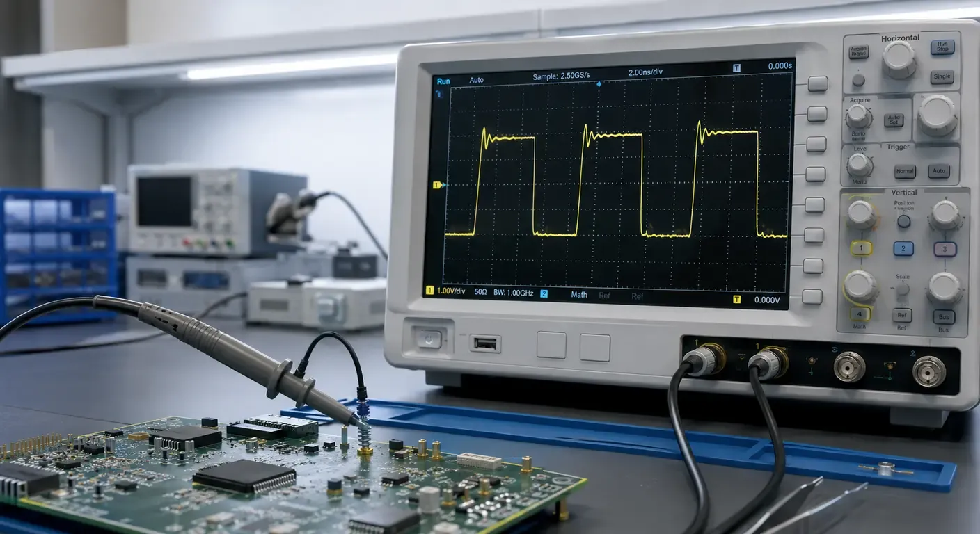
Bandwidth is the first specification on almost every oscilloscope datasheet, and the one most often misread. It looks like a simple statement of the highest frequency the instrument can measure. It is not.
A more useful way to think about it is this: bandwidth marks the point where an oscilloscope stops telling the truth about a signal. Well below that frequency, what appears on screen closely matches reality. As the signal approaches it, amplitudes shrink, edges soften, and fast details quietly disappear.
That last point is what makes the specification worth understanding. A bandwidth-limited measurement rarely looks wrong — it looks clean. Ringing fades, overshoot flattens, and a marginal design can appear perfectly healthy. The oscilloscope gives no warning that it is filtering the very behaviour you are trying to observe.
This guide explains oscilloscope bandwidth from both directions: what the specification actually means, and what it changes on the bench. It covers the −3 dB definition, the effect of bandwidth on amplitude, shape and timing, the relationship with sample rate and rise time, and a practical method for selecting bandwidth — including the probe and accessories, which frequently set the real limit long before the instrument does.
Oscilloscope bandwidth is one of the key concepts covered in our Test & Measurement: Complete Guide to Electronic Test Equipment resource, which explores the wider range of tools and measurement techniques used by engineers.
What Is Oscilloscope Bandwidth?
The definition of bandwidth
Oscilloscope bandwidth describes the frequency range over which the instrument reproduces an input signal within a specified amplitude accuracy. It is a property of the entire analog signal path — input connector, attenuator, front-end amplifier and the analog-to-digital converter that follows.
Bandwidth is expressed as a single frequency, for example 200 MHz or 1 GHz. That figure is the upper limit of a low-pass response. Below it, signals pass with progressively less error. Above it, attenuation increases rapidly and waveform details become progressively less representative of the original signal.
One consequence follows directly from this definition, and it is the source of most measurement errors: bandwidth is not a threshold where measurement suddenly stops working. The response rolls off gradually, so meaningful error exists long before the specified frequency is reached.
What the −3 dB point means
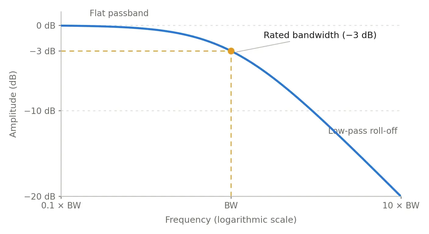
By convention, oscilloscope bandwidth is specified at the −3 dB point: the frequency at which a sine wave applied to the input is displayed at approximately 70.7% of its actual amplitude.
The figure comes from the decibel definition. A voltage ratio of −3 dB corresponds to a factor of 0.707, equivalent to half the power. A 1 V peak-to-peak sine wave at the bandwidth frequency is therefore displayed as roughly 707 mV peak-to-peak — an amplitude error of about 30%.
Why manufacturers specify bandwidth this way
The −3 dB convention is inherited from filter and amplifier design, where it provides a single, repeatable and vendor-neutral figure of merit. Because every oscilloscope front end behaves as a low-pass filter, specifying the half-power frequency lets different instruments be compared on the same basis.
The shape of the roll-off, however, depends on the instrument design. Oscilloscopes up to roughly 1 GHz typically exhibit a Gaussian-like response, where attenuation increases smoothly and continues well beyond the −3 dB point. Higher-bandwidth instruments more often use a maximally flat response, which stays closer to 0 dB across most of the band and then falls sharply.
Two oscilloscopes with the same −3 dB figure can therefore behave quite differently near the limit. A flat-response instrument holds amplitude accuracy closer to its rated bandwidth but rejects out-of-band content more abruptly, while a Gaussian instrument degrades earlier and more gently.
Datasheets also qualify the bandwidth figure in ways that are easy to overlook. Full bandwidth is often guaranteed only at vertical settings of 10 mV/div and above; at the most sensitive settings, such as 1 mV/div or 2 mV/div, the specified bandwidth may be significantly lower. Reading the specification footnotes is part of understanding any instrument, as discussed in our guide to oscilloscope specifications and what they actually mean.
The frequency response below shows how an oscilloscope behaves as a low-pass system.
Why Bandwidth Is Important for Oscilloscope Measurements
Signal attenuation
The most direct effect of limited bandwidth is amplitude error. For an instrument with a Gaussian response, a sine wave at one third of the specified bandwidth is typically displayed with roughly 3% error, and at one fifth of the bandwidth with roughly 1 to 2%. These figures are the origin of the selection rules discussed later in this article.
Attenuation is often the least visible error, because a waveform that is 10% too small still looks entirely plausible on screen. Voltage measurements, power calculations and design margin analysis are all affected without any visual warning.
Waveform distortion
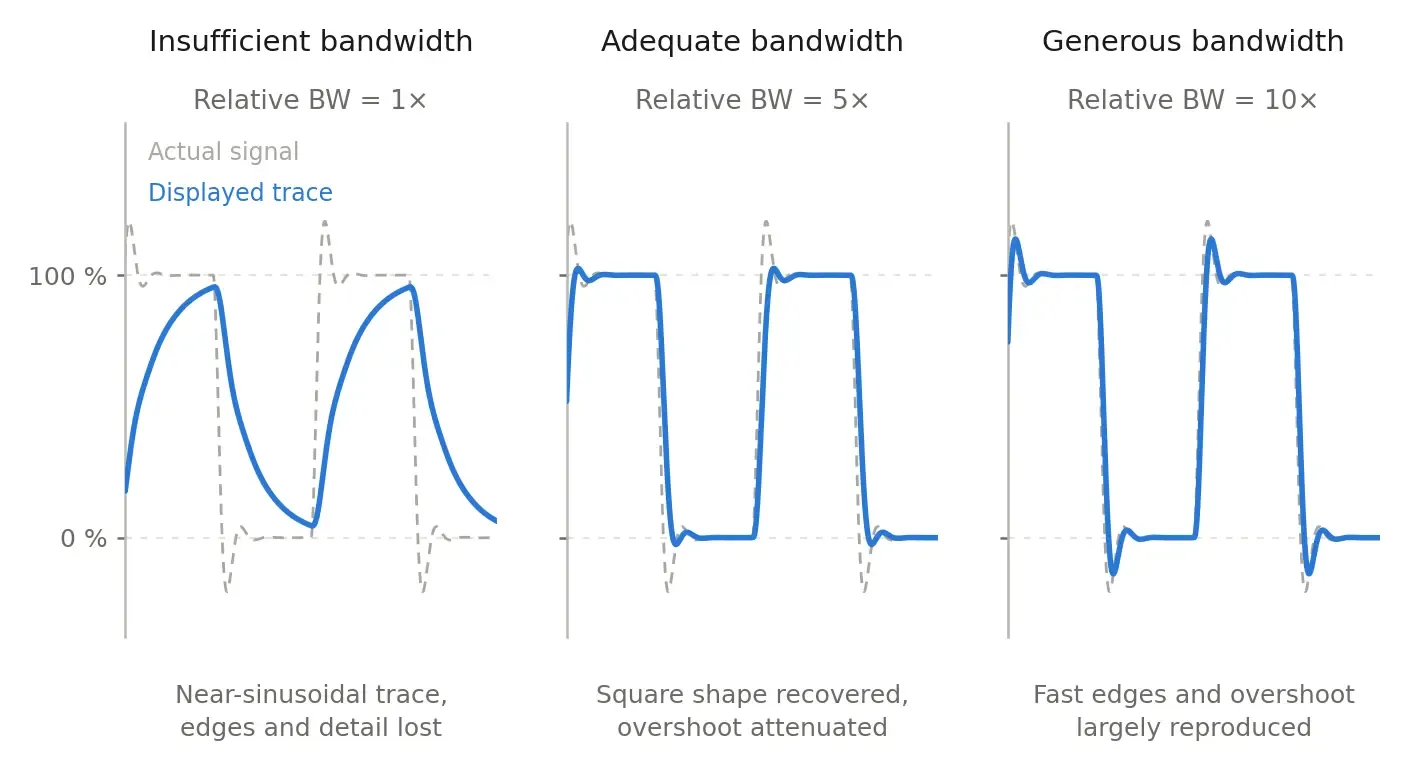
Non-sinusoidal signals consist of a fundamental frequency plus harmonics. A bandwidth limit attenuates the higher harmonics more than the fundamental, so it changes the shape of the waveform, not only its size.
On the bench this appears as:
- rounded corners on square waves
- slower apparent transitions
- reduced overshoot
- suppressed or missing ringing
- narrow glitches shrunk in amplitude, or absent entirely
Insufficient bandwidth therefore makes signals look better behaved than they are — a particularly dangerous failure mode during debugging, because it hides exactly the anomalies you are looking for.
Measurement accuracy
Automated measurements inherit every error present in the acquired waveform. Rise time, fall time, overshoot, pulse width and slew rate all depend on the reproduced edge shape. If the instrument slows the edge, the reported rise time describes the oscilloscope as much as the circuit.
Frequency-domain functions are affected in the same way. An FFT computed from a bandwidth-limited acquisition shows attenuated high-frequency content, which can lead to wrong conclusions during EMI investigation or harmonic analysis.
How Oscilloscope Bandwidth Affects Different Signal Types
Sine waves
A sine wave contains a single frequency component, so bandwidth affects amplitude only — the shape stays sinusoidal regardless of attenuation. This is the simplest case, and the reason the −3 dB specification is defined using sine waves. Selecting bandwidth here requires only enough margin to keep amplitude error acceptable.
Square waves
An ideal square wave contains the fundamental plus all odd harmonics, with amplitude decreasing as harmonic order increases. Reproducing a recognisable square shape requires several harmonics; capturing edge detail requires many more.
Displaying a square wave with reasonable fidelity generally requires bandwidth covering at least the fifth harmonic, while accurate edge and overshoot analysis typically calls for the tenth harmonic or beyond. A 10 MHz square wave analysed for edge behaviour therefore demands far more than 10 MHz of bandwidth.
Pulse signals
Pulses are characterised by their edges and their width rather than by a repetition frequency. A narrow pulse spreads energy across a wide frequency range, and the shorter the pulse, the wider that range.
An oscilloscope with insufficient bandwidth both reduces pulse amplitude and widens the apparent pulse. Short glitches may appear at a fraction of their real amplitude, or fail to appear at all. For pulse work, bandwidth should always be derived from the transition time, never from the repetition rate.
High-speed digital signals
For digital signals, clock frequency is a poor predictor of required bandwidth. The relevant parameter is the edge rate. A widely used engineering approximation defines a knee frequency, above which the spectral content of an edge falls off rapidly:
f_knee ≈ 0.5 / tr
where tr is the 10% to 90% rise time, or 0.4 / tr for a 20% to 80% figure. A 1 ns edge corresponds to a knee frequency of roughly 500 MHz, whether the signal toggles at 10 MHz or 100 MHz. Reliable measurement of edge shape, overshoot and ringing requires bandwidth of 1.0 to 1.9 times the knee frequency, by timing accuracy and response shape.
This is why a slow bus driven by very fast devices can demand more bandwidth than a faster bus built from slower ones.
The comparison below shows how the same fast square wave appears when measured with insufficient, adequate and generous oscilloscope bandwidth.
Oscilloscope Bandwidth vs Sample Rate
Bandwidth is only half of an oscilloscope’s ability to capture a fast signal. The second half is sample rate, and the two are routinely confused.
Why these specifications are different
Bandwidth is an analog property. It describes how faithfully the front end passes a signal before digitisation. Sample rate, expressed in samples per second, is a digital property: how often the ADC captures a value.
The two are independent. A high sample rate cannot restore frequency content the analog front end has already attenuated, and a wide analog bandwidth is wasted if the signal is sampled too sparsely to reconstruct it.
| Aspect | Bandwidth | Sample rate |
|---|---|---|
| Domain | Analog front end | Digitisation |
| Unit | Hz | Samples per second |
| Limits | Amplitude and shape fidelity | Waveform reconstruction and timing detail |
| Typical failure | Attenuated, rounded waveforms | Aliasing, missed events |
How they work together
Nyquist theory states that sampling must exceed twice the highest frequency component to avoid aliasing. Oscilloscope measurements usually require additional margin because real signals are not perfect sine waves and reconstruction depends on the instrument architecture. Instruments using sin(x)/x interpolation typically specify a sample rate of around 2.5 times the bandwidth as a minimum, while 4 to 5 times is preferable for single-shot acquisitions, pulse work and linear interpolation.
Sample rate also depends on how the instrument is configured. Many oscilloscopes interleave ADC resources, so the maximum rate is available only on a reduced number of channels. Enabling all channels may halve the effective rate — which matters when capturing fast edges on several signals at once. Our articles on oscilloscope sample rate and memory depth cover this interaction in more detail.
Common misconceptions
- A high sample rate compensates for low bandwidth. It does not. Attenuation happens before sampling and cannot be undone afterwards.
- Sample rate defines the highest measurable frequency. Sample rate sets the reconstruction limit; bandwidth sets the analog limit. Whichever is lower governs the result.
- The advertised sample rate is always available. Channel interleaving and memory depth both influence the rate actually used at a given timebase setting.
Oscilloscope Bandwidth vs Rise Time
Understanding rise time
Rise time is the interval a signal needs to transition between two defined amplitude levels — conventionally 10% and 90% of the final value. Some high-speed standards use 20% to 80% instead, so the reference levels should always be checked before comparing figures.
Oscilloscopes have a rise time of their own, set by their bandwidth. This instrument rise time defines the fastest transition the oscilloscope can display, whatever signal is applied to it.
The bandwidth–rise time relationship
For instruments with a Gaussian response, bandwidth and rise time are linked by a simple approximation:
BW × tr ≈ 0.35
The constant depends on the instrument design. Oscilloscopes with a maximally flat response, common above 1 GHz, use values closer to 0.40 or 0.45. The manufacturer’s specified rise time should always take precedence over a calculated one.
Approximate oscilloscope rise time derived from bandwidth (Gaussian response, k = 0.35)
- 100 MHz
- ≈ 3.5 ns
- 200 MHz
- ≈ 1.75 ns
- 500 MHz
- ≈ 700 ps
- 1 GHz
- ≈ 350 ps
- 2 GHz
- ≈ 175 ps (often slower in practice; flat-response instruments use k ≈ 0.40–0.45)
Because the instrument and the signal both contribute to the observed transition, the measured rise time is approximately the root-sum-square of the two:
tr_measured ≈ √(tr_signal² + tr_scope²)
If a 1 ns signal edge is measured with an oscilloscope whose rise time is also 1 ns, the display shows about 1.41 ns. The instrument has added 41% error to a fundamental timing parameter. Keeping the oscilloscope rise time at roughly one third of the signal rise time reduces that contribution to a few percent.
Why both specifications matter
Bandwidth is the natural way to reason about amplitude error and frequency content. Rise time is the natural way to reason about timing measurements and edge fidelity. They describe the same physical limitation from two directions, and instrument selection usually needs both: bandwidth to confirm harmonic content is preserved, rise time to confirm timing measurements remain credible. Our dedicated article on oscilloscope rise time and edge measurement works through this in more depth.
How Much Bandwidth Do You Really Need?
General selection rules
Choosing oscilloscope bandwidth comes down to one question: is the signal defined by its frequency, or by its edges?
If the signal is essentially sinusoidal or narrowband, work from frequency. Select bandwidth of at least three times the highest frequency component for approximately 3% amplitude error, or five times for approximately 1 to 2%.
If the signal is digital or pulsed, work from the fastest edge in the system — not the clock. Calculate the knee frequency as above, then select bandwidth of 1.0 to 1.9 times that value. The rise time rule gives the same answer from the other direction: choose an instrument whose rise time is about one third of the signal rise time.
| Signal type | Selection method | Practical guidance |
|---|---|---|
| Sine and narrowband | 3× to 5× the highest frequency component | 3× for approximately 3% amplitude error, 5× for 1 to 2% |
| Digital signals | 1.0× to 1.9× the knee frequency | Use the fastest edge in the system, not the clock rate |
| Pulses and glitches | Derive from transition time, never repetition rate | Also verify sample rate and memory depth for single-shot capture |
| Power switching | Set by device transition time and gate-loop ringing | Bandwidth is secondary to voltage rating, isolation and common-mode rejection |
| RF-related | Depends on whether the measurement concerns the carrier, modulation envelope, harmonics or transient behaviour | Narrowband spectral analysis is usually better served by a spectrum analyser |
Excess bandwidth is not free. A wider front end admits more broadband noise, raising the noise floor and reducing effective resolution on small signals. The bandwidth limit filter found on most instruments, typically 20 MHz, exists precisely for this reason and should be used whenever the signal of interest sits well below that limit.
Examples by application
The figures below are practical starting points, not requirements.
| Application | Common starting points (application dependent) | Reasoning |
|---|---|---|
| Embedded electronics | 100–200 MHz | MCU clocks, I²C, SPI and UART are slow, but logic edges of a few nanoseconds set the real requirement |
| Power electronics | 100–500 MHz | Switching frequencies are low, yet SiC and GaN transitions of a few nanoseconds and gate-loop ringing demand high-frequency response |
| Automotive electronics | 100–200 MHz | CAN, CAN FD and LIN are low-rate; automotive Ethernet variants require GHz-class instruments and dedicated probing |
| RF systems | Depends on whether the measurement concerns the carrier, modulation envelope, harmonics or transient behaviour | Oscilloscopes are used here for envelope, pulsed and transient behaviour rather than narrowband spectral measurement |
| High-speed digital communications | 2 GHz and above | Interfaces with sub-nanosecond edges require substantial bandwidth, deep memory and active or differential probing |
These values are only general references. Actual bandwidth requirements depend primarily on edge rate and measurement objective.
Bandwidth is one criterion among several. For the full selection process, including vertical resolution, memory depth and triggering, see our guide on how to choose an oscilloscope.
Factors That Can Limit Effective Bandwidth
Probe bandwidth
The probe is part of the measurement path, and its bandwidth is frequently lower than the oscilloscope’s. A general-purpose 10:1 passive probe presents roughly 10 to 15 pF of input capacitance, and its input impedance falls as frequency rises, loading the circuit under test.
Passive probes are typically practical to a few hundred megahertz, depending on probe design and measurement conditions. Beyond that, active single-ended or differential probes with input capacitance near 1 pF become necessary — both for bandwidth and to limit circuit loading. Probes must also be compensated before use; an uncompensated probe distorts edge shape regardless of its bandwidth rating. Our overview of oscilloscope probes and probing techniques covers probe types and their trade-offs.
Test leads and accessories
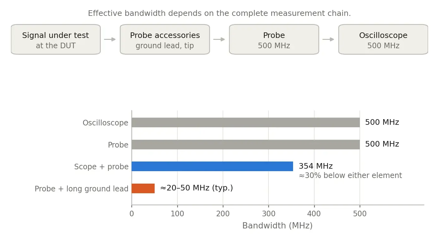
Accessories often limit performance more than the probe itself. The long alligator-clip ground lead supplied with most probes forms an inductive loop with the probe capacitance, creating a resonant circuit that produces ringing and can restrict usable bandwidth to a few tens of megahertz.
Replacing that lead with a short ground spring, keeping the loop area minimal and probing directly at the point of interest often improves measured edge quality more than upgrading the instrument. Adapters, extension cables and unterminated coaxial connections cause similar degradation.
Overall measurement system bandwidth
The bandwidth of a complete measurement chain is always lower than that of any individual element. For systems with approximately Gaussian responses, the combination can be estimated as:
1 / BW_system² ≈ 1 / BW_scope² + 1 / BW_probe²
A 500 MHz oscilloscope used with a 500 MHz probe yields a system bandwidth of approximately 354 MHz. Pairing a probe with an instrument of the same rating therefore costs roughly 30% of the expected performance. This is why manufacturers specify probe and oscilloscope combinations together — and why the system figure, not the instrument figure, is the one that matters.
Common Mistakes When Choosing Oscilloscope Bandwidth
- Selecting bandwidth from clock frequency. Edge rate determines spectral content, and a slow bus with fast drivers can require more bandwidth than a faster one.
- Ignoring the probe. Instrument bandwidth means little if the probing solution cannot deliver the signal to the input.
- Using the supplied ground lead for fast edges. The resulting resonance produces ringing that is easily mistaken for a circuit problem.
- Assuming sample rate compensates for bandwidth. The two specifications address different limitations, and neither substitutes for the other.
- Working close to the specified bandwidth. Amplitude error reaches roughly 30% at the −3 dB point, and significant error exists well below it.
- Over-specifying bandwidth for low-frequency work. Additional bandwidth adds noise, which degrades resolution on small signals.
- Overlooking datasheet conditions. Bandwidth may be reduced at the most sensitive vertical settings, and maximum sample rate may require a reduced channel count.
- Trusting a clean waveform. Bandwidth limitations remove anomalies rather than adding them, so an unexpectedly clean signal deserves scrutiny.
Frequently Asked Questions
What is oscilloscope bandwidth?
Oscilloscope bandwidth is the frequency range over which the instrument reproduces a signal within a specified amplitude accuracy. It is set by the analog signal path and stated as the frequency where the displayed amplitude has fallen by 3 dB relative to low-frequency response. Beyond that point, the displayed waveform becomes increasingly affected by attenuation and distortion.
Why is oscilloscope bandwidth important?
Insufficient bandwidth attenuates high-frequency content. Amplitudes read low, edges round off, rise times appear slower, and glitches, ringing and overshoot can vanish. Because these limitations make signals look cleaner rather than worse, they give no visual warning, so genuine circuit problems can be missed entirely during debugging.
What does the −3 dB bandwidth mean?
The −3 dB point is the frequency at which an applied sine wave is displayed at approximately 70.7% of its true amplitude, corresponding to half the power. A signal measured at the rated bandwidth therefore already shows roughly 30% amplitude error, which is why practical measurements should be made well below that frequency.
What is the difference between bandwidth and sample rate?
Bandwidth is an analog specification describing how faithfully the front end passes a signal before digitisation. Sample rate is a digital specification describing how often that signal is measured. A high sample rate cannot recover content the front end has already attenuated, so both must be adequate for a valid measurement.
How much oscilloscope bandwidth do I need?
For sinusoidal signals, choose at least three times the highest frequency component for about 3% amplitude error, or five times for 1 to 2%. For digital and pulse signals, calculate the knee frequency as 0.5 divided by a 10-90% rise time, or 0.4 for a 20-80% one, and take 1.0 to 1.9 times that value. Alternatively, select an instrument whose rise time is about one third of the signal rise time.
Does the oscilloscope probe affect bandwidth?
Yes. The probe, its ground connection and any adapters form part of the measurement system, and the combined bandwidth is normally lower than that of the individual elements. A 500 MHz probe on a 500 MHz oscilloscope gives approximately 354 MHz of system bandwidth, and a long ground lead can reduce usable bandwidth much further.
Related articles
Electronics18 min read
Function Generator vs Arbitrary Waveform Generator: What You Are Buying
Three names, two architectures: how DDS and point-by-point playback differ, what the labels hide, and how to read the architecture off a datasheet.
Electronics23 min read
How to Choose a Signal Generator: Getting the Signal You Asked For
How to turn a required stimulus into datasheet requirements: the load the instrument assumes, bandwidth against sample rate, reconstruction and vertical resolution.
Electronics22 min read
How to Choose a Multimeter: A Specification-Led Buying Guide
Choose a multimeter by the errors it introduces: burden voltage, input loading, AC bandwidth, safety category and accuracy on the reading you actually take.
Electronics16 min read
How to Use a Thermal Camera: Getting Readings You Can Trust
A thermal camera always shows a number. Learn the checks — emissivity, reflected temperature, focus and spot size — that decide whether it is a measurement.