Sample Rate Explained: How Oscilloscopes Capture Digital Waveforms
Learn how oscilloscope sample rate affects waveform accuracy and aliasing, and how to read the figure correctly on a datasheet. Understand Sa/s and sampling fundamentals.
By YDT EditorialUpdated 22 min read
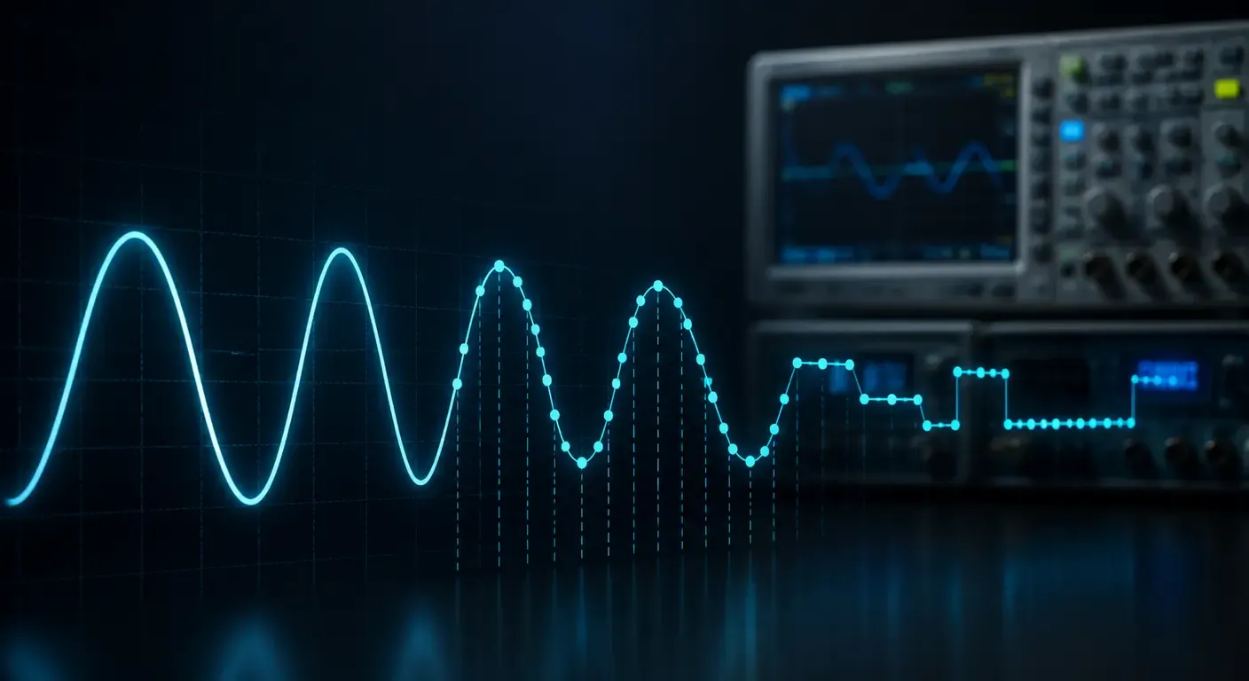
Sample rate is the number of times per second a digital instrument measures an analog signal. Every digital measurement instrument has to solve the same problem: the physical world produces continuous signals, and digital electronics can only work with discrete numbers. Sample rate is the specification that describes how that conversion happens in time.
The consequences are practical rather than theoretical. Sample rate is one of the factors that determines whether a glitch is captured or missed, whether a rise time measurement is meaningful, and whether the waveform on screen represents the signal that actually exists on the board. Bandwidth, probing and signal integrity also play a critical role. It is one of the first specifications engineers look at when selecting an oscilloscope or a data acquisition system, and one of the most frequently misinterpreted.
This guide explains what sample rate means, how it relates to signal frequency, what happens when it is too low, how to read the specification correctly on a datasheet, and how to choose an appropriate value for a given measurement task.
Sample rate is one specification among several that decide whether a measurement can be trusted. Our complete Test & Measurement guide places it alongside bandwidth, resolution and memory depth, and covers the rest of the instruments on a bench.
What Is Sample Rate?
Definition of Sample Rate in Digital Measurement
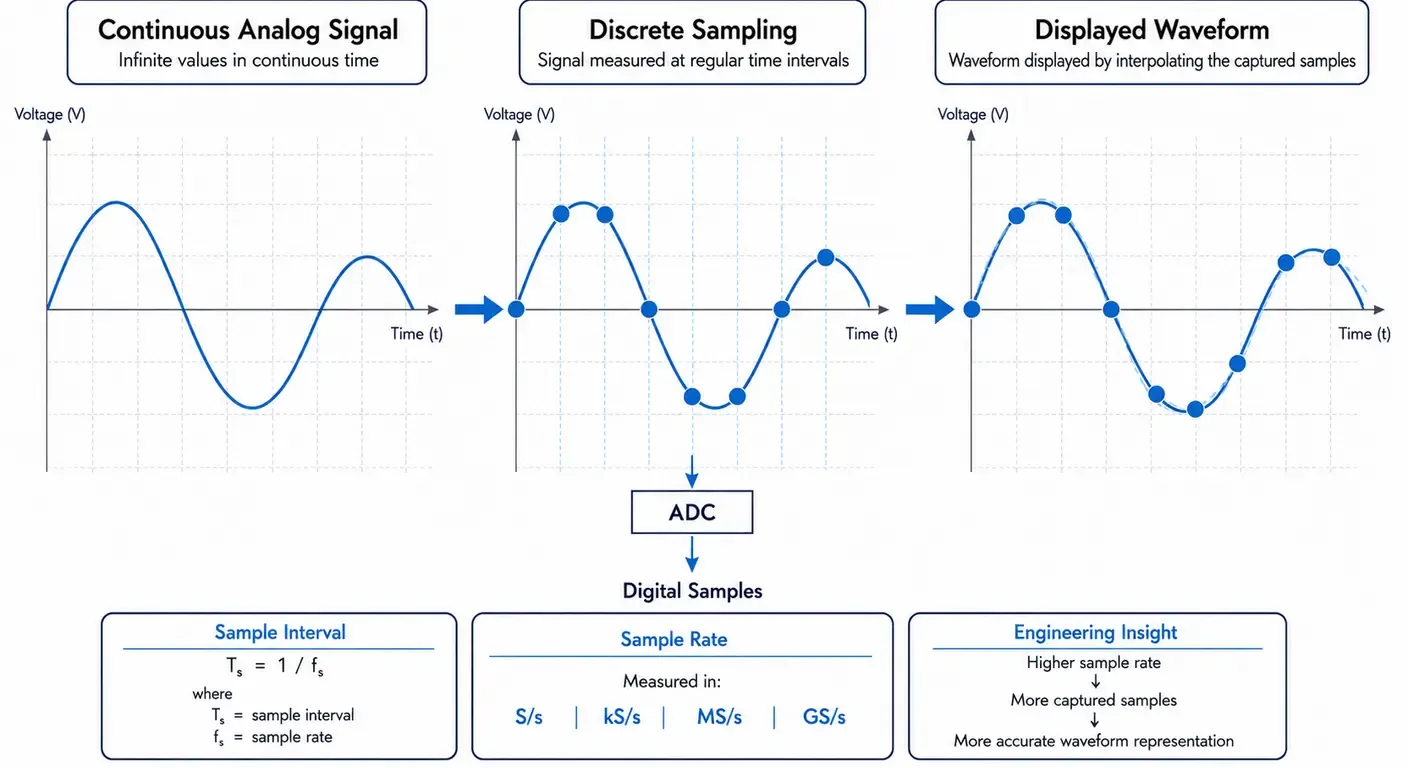
Sample rate, also called sampling rate or sampling frequency, is the number of individual measurements an instrument takes from an analog signal in one second. Each measurement is called a sample, and the rate at which samples are collected is expressed in samples per second.
The units follow standard SI prefixes:
- S/s — samples per second
- kS/s — thousand samples per second
- MS/s — million samples per second
- GS/s — billion samples per second
For example, an instrument specified at 1 MS/s collects one million samples every second, meaning one measurement every microsecond. An oscilloscope specified at 5 GS/s collects five billion samples per second, or one sample every 200 picoseconds.
The reciprocal of the sample rate is the sample interval, which is often the more useful number when reasoning about timing. If you need to resolve an event lasting 10 ns with several points, a sample interval of 200 ps gives you roughly fifty samples across that event. A sample interval of 20 ns gives you none.
How Analog Signals Become Digital Data
An analog signal is continuous in both time and amplitude. It has a defined value at every instant. A digital measurement system cannot store an infinite number of values, so it inspects the signal at regular intervals and records the amplitude at each of those instants.
The component responsible for this is the analog-to-digital converter, or ADC. On each clock edge of the sampling process, the ADC measures the instantaneous voltage present at its input and converts it into a numeric code. The instrument then stores that code in acquisition memory.
What appears on screen afterwards is not the original signal. It is a reconstruction built from the stored samples, usually with an interpolation algorithm that draws a plausible curve between them. How faithful that reconstruction is depends on how many samples were captured per cycle, and on which interpolation method the instrument applies.
Why Is Sample Rate Important in Test and Measurement?
Capturing Signal Details
Signals rarely fail in convenient ways. The events engineers most need to see are usually short: a runt pulse on a bus, a ringing artifact after a switching transition, a narrow glitch that triggers a spurious reset, an ESD event coupling into a sensor line.
These features exist for a limited time. If no sample falls within that window, the instrument has no record that the event occurred. This applies to:
- Fast transitions, where the rise or fall time carries the information of interest
- Narrow pulses, which may be shorter than the sample interval
- Transient events, which occur once and cannot be averaged or repeated
- Noise analysis, where high-frequency content is the subject of the measurement
A higher sample rate increases the density of measurement points in time, which increases the probability that short-lived behaviour is captured and reduces the interpolation error in the displayed waveform.
Impact on Measurement Accuracy
Sample rate strongly affects how well a waveform is represented, and automated measurements are derived from that representation. Rise time, pulse width, period, duty cycle and peak values are all calculated from stored sample points. If the sample density is low, those calculations are performed on an approximation and inherit its error.
The distinction matters when reading datasheets. Two instruments with identical sample rates can produce measurably different results because their analog front ends, ADC resolution and noise floors differ.
Sample Rate vs Frequency: Understanding the Relationship
The Nyquist Sampling Theorem Explained
The Nyquist-Shannon sampling theorem defines the condition under which a bandlimited signal can be reconstructed from its samples without ambiguity:
Sample Rate ≥ 2 × Highest Frequency ComponentTwo related terms are frequently used interchangeably and should not be. The Nyquist rate is the minimum acceptable sample rate, equal to twice the highest frequency component in the signal. The Nyquist frequency is half of whatever sample rate the instrument is actually running at. Any signal content above the Nyquist frequency cannot be correctly represented in the sampled data.
The relationship is normally written with a greater-than-or-equal sign, but the boundary case is degenerate: a sine wave sampled at exactly twice its frequency yields a recovered amplitude that depends on where the samples happen to fall relative to the peaks, and can in principle be zero. Practical work treats twice the maximum frequency as a limit to stay clear of, not a target.
Two further qualifications are essential.
First, the theorem refers to the highest frequency component present in the signal, not the frequency the engineer is interested in. A 1 MHz square wave contains harmonics extending far beyond 1 MHz. Wideband noise, coupled interference and switching transients all count as signal content for the purposes of the theorem.
Second, the theorem describes mathematical reconstruction under ideal conditions, using perfect interpolation and assuming the input has been strictly bandlimited before sampling. Real instruments approximate both. Satisfying Nyquist guarantees that the information is mathematically recoverable; it does not guarantee that the waveform on screen is usable for the measurement at hand.
Why Engineers Choose Higher Sample Rates
Beyond satisfying the theorem, oversampling delivers practical benefits:
- Waveform detail. More points per cycle produce a display that requires less interpolation and is easier to interpret visually.
- Unexpected behaviour. Faults rarely announce their bandwidth in advance. Headroom in sample rate allows anomalies outside the expected frequency range to appear rather than being filtered into invisibility.
- Harmonic content. Analysing distortion, switching behaviour or signal integrity requires capturing harmonics several times above the fundamental.
- Single-shot events. A transient cannot be re-measured. Whatever the instrument captured on that acquisition is all the information that will ever exist.
- Post-processing headroom. Digital filtering, FFT analysis and decimation all benefit from a denser original data set.
What Happens When Sample Rate Is Too Low?
Understanding Aliasing
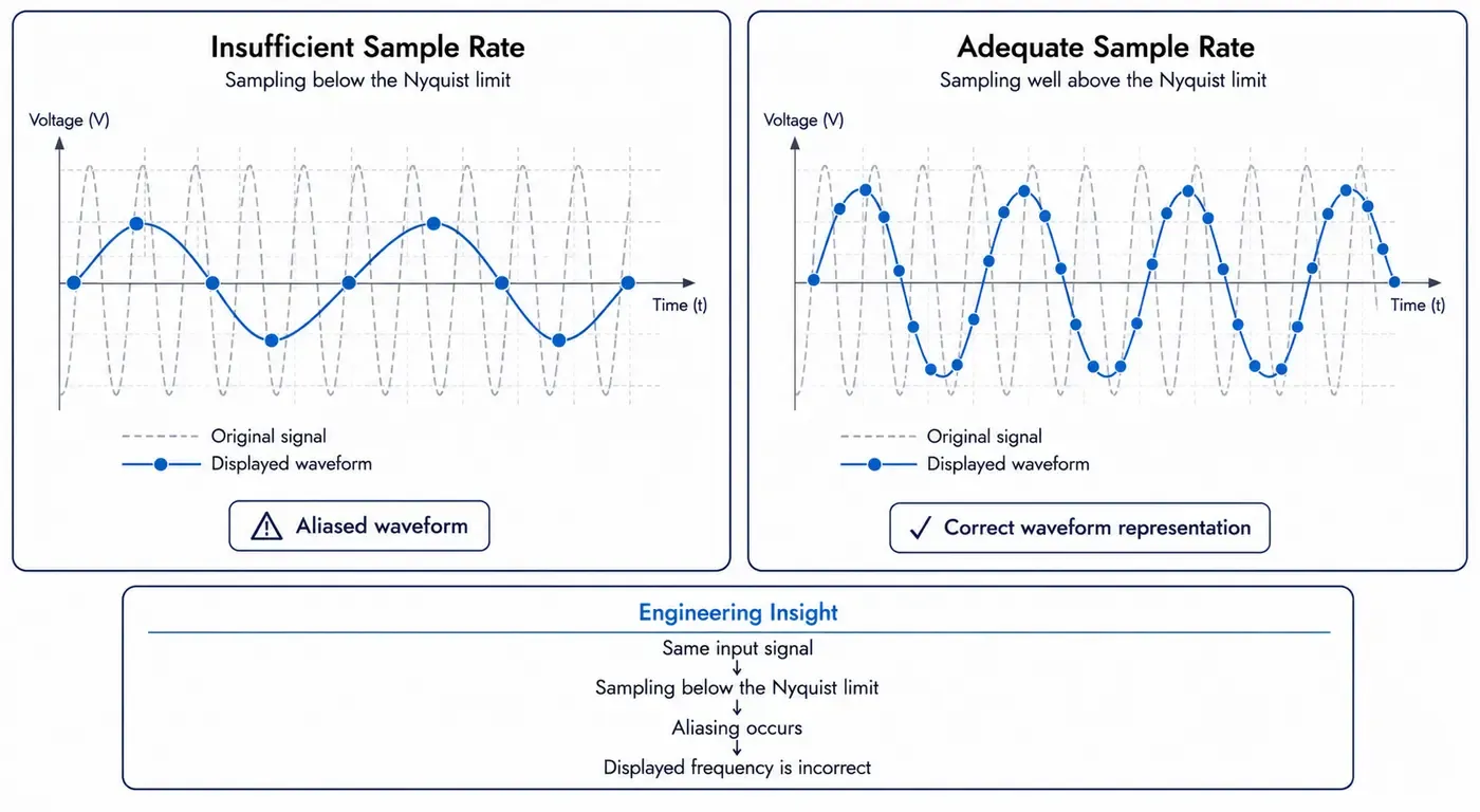
Aliasing occurs when a signal contains frequency components above the Nyquist frequency. Those components do not disappear from the data. They are folded back into the measurable range and appear as lower-frequency content that was never present in the original signal.
The resulting frequency is the difference between the actual signal frequency and the nearest integer multiple of the sample rate. A 6 kHz sine wave sampled at 10 kS/s has a Nyquist frequency of 5 kHz, so the 6 kHz component is displayed at 4 kHz. The waveform on screen is stable, clean and entirely wrong.
Instrument classes handle this risk differently, and the difference is worth understanding. Data acquisition systems intended for spectral or sensor measurements typically place a dedicated analog anti-aliasing filter ahead of the ADC, so that content above the Nyquist frequency is attenuated before conversion. Many general-purpose oscilloscopes do not rely on a dedicated steep anti-aliasing filter; they rely instead on the roll-off of the analog front end and on running the ADC far above the Nyquist rate. That is one reason an oscilloscope operating at a slow timebase, where the sample rate has been automatically reduced, is more exposed to aliasing than the headline sample rate suggests.
Once aliasing has occurred, it cannot be undone in software. The original and the alias are indistinguishable in the stored data.
Lost Signal Information
Aliasing is the most discussed failure mode, but simple loss of detail is more common in day-to-day bench work. When the sample interval is comparable to the features being measured, the instrument records:
- Attenuated peaks, because no sample coincided with the actual maximum of a narrow pulse
- Incorrect timing, because edge positions are resolved only to within one sample interval
- Missing events, because a short glitch fell entirely between two samples
- Distorted edges, where a genuine transition is represented by too few points to characterise its shape
Automated measurements will still return values under these conditions. They will simply be wrong, with no warning to the operator.
How to Choose the Right Sample Rate
Start With the Maximum Signal Frequency
Selection begins with an honest estimate of the highest frequency content the measurement must capture, not the nominal frequency of the signal. Consider:
- The fundamental frequency of the signal
- The harmonics required for the measurement to be meaningful, which for square waves and digital signals extend well beyond the fundamental
- Edge rates, which for digital signals usually dominate the bandwidth requirement regardless of clock frequency
- Noise and interference components that may be relevant or may need to be filtered out before sampling
- Expected anomalies, including transients that are the actual object of the investigation
For digital signals, the rise time is the governing parameter. Consider a 10 MHz clock with a 1 ns rise time. The clock frequency suggests a modest instrument, but the edge does not. Because instrument and signal rise times combine approximately as a root-sum-square, an oscilloscope rise time of roughly one third of the signal rise time keeps the measurement error in the region of a few percent. That implies an instrument rise time near 330 ps, which corresponds to about 1 GHz of bandwidth. A sample rate of 5 GS/s provides a 200 ps sample interval. This is sufficient to represent the timing scale involved, but detailed edge characterisation generally benefits from additional samples across the transition. Selecting on the 10 MHz clock frequency instead would have produced a measurement with no useful edge information at all.
Consider Signal Type and Application
Different application areas emphasise different aspects of the sampling requirement:
| Application | Important Consideration |
|---|---|
| Digital electronics | Edge rates and short glitches rather than clock frequency |
| Embedded systems | Bus timing, setup and hold margins, and infrequent protocol anomalies |
| Audio signals | A defined and limited frequency band with strong anti-alias filtering |
| Power electronics | Fast switching transitions superimposed on low-frequency waveforms |
| Motor control | Long observation windows containing short, repetitive switching events |
| RF and communications | High carrier frequencies, often handled through downconversion before sampling |
| Sensor and process monitoring | Low bandwidth, long capture duration, and resolution over speed |
Power electronics and motor drives illustrate the tension particularly well. The fundamental may be 50 Hz or a few tens of kilohertz, while the turn-off transition of a MOSFET or IGBT occurs in tens of nanoseconds and is often followed by ringing at much higher frequencies. Capturing the switching edge demands a high sample rate; characterising behaviour across a motor start-up sequence demands a capture window measured in tens or hundreds of milliseconds. Both requirements apply to the same investigation.
Balance Sample Rate With Memory Depth
Sample rate and acquisition memory are inseparable. Memory depth determines how many samples can be stored, and the two together determine how long a window of time can be captured:
Capture Time = Memory Depth ÷ Sample RateAn instrument with 10 Mpts of memory running at 5 GS/s can capture 2 ms of signal. The same memory at 1 MS/s covers 10 seconds. This is why many oscilloscopes automatically reduce the sample rate as the timebase is slowed: memory is finite, and the instrument trades temporal resolution for capture duration. Our dedicated guide to oscilloscope memory depth covers how that depth is allocated across channels and what happens when it runs out.
The motor drive case above makes the constraint concrete. Observing 100 ms of operation at 1 GS/s would require 100 Mpts of memory on a single channel, which is beyond most general-purpose instruments once several channels are active. Segmented memory acquisition is the usual answer: the instrument stores only short windows around each trigger event and discards the intervals between them, preserving the sample rate where it matters without paying for the dead time.
Verify How the Specification Is Stated
Headline sample rate figures are frequently quoted under favourable conditions. Before comparing instruments, confirm the following in the datasheet rather than in the marketing summary:
- Is the rate per channel or shared? Many oscilloscopes and digitizers interleave their ADCs, so an instrument rated at 2 GS/s on one channel may provide 1 GS/s per channel when two channels are active. Interleaved memory behaves the same way.
- Does it apply to all acquisition modes? High-resolution, averaging, peak-detect and segmented modes may each impose different limits.
- What memory depth accompanies it? Maximum sample rate combined with shallow memory produces a capture window too short to be useful at realistic timebase settings.
- Is the front end capable of using it? A sample rate far in excess of what the instrument bandwidth can pass adds data volume, not information.
- Is the figure real-time or interpolated? Some specifications quote an effective rate that assumes a repetitive signal.
Sample Rate in Common Test Equipment
Sample Rate in Oscilloscopes
Sample rate is one of the defining specifications of a digital storage oscilloscope, alongside bandwidth and memory depth. In real-time sampling mode, the instrument acquires the entire waveform in a single pass, which is the only viable approach for non-repetitive events.
An additional mode, equivalent-time sampling, builds a high-resolution picture of a repetitive signal by combining samples taken at different points across many cycles. This produces an effective sample rate far above the instrument’s real-time capability, but it requires a stable, repeating signal and is unusable for single-shot capture. It is therefore of no help when hunting an intermittent fault.
The relationship between bandwidth and sample rate is fixed at design time. A high-bandwidth front end is only useful if the ADC behind it samples fast enough to represent the frequencies that front end passes. Instruments are normally specified so that the two are consistent, which is why comparing sample rates across models with different bandwidths tells you very little on its own.
Sample Rate in Data Acquisition Systems
DAQ hardware covers a much wider range than the oscilloscope category, and generalisation is unreliable. Many general-purpose DAQ front ends operate from a few samples per second to a few hundred kS/s per channel and prioritise resolution, channel count, long-term stability and continuous acquisition over speed. High-speed digitizer cards, transient recorders and instrumentation intended for physics or power quality work operate at MS/s to GS/s rates and overlap directly with oscilloscope territory. The correct approach is to read the specification for the specific product rather than to assume a class behaviour.
Typical requirements in the lower-speed segment include:
- Sensor measurements, where thermocouples, strain gauges and pressure transducers change slowly
- Industrial monitoring, where continuous acquisition over hours or days matters more than temporal resolution
- Data logging, where storage volume is a direct function of sample rate and channel count
Many precision DAQ front ends use delta-sigma ADCs, which sample at a high internal rate, shape quantisation noise out of the band of interest, and then filter and decimate to the configured output rate. This yields high effective resolution and inherent anti-alias filtering, at the cost of a fixed group delay through the digital filter and a limited maximum output rate.
Multiplexed systems deserve particular attention. When one ADC is shared across several channels, the specified aggregate sample rate is divided among them, and channels are not sampled simultaneously. Where phase relationships between channels matter, as in power measurement or vibration analysis, simultaneous-sampling hardware is required.
Sample Rate in Other Instruments
Sample rate governs the behaviour of most modern digital instruments:
- Signal and spectrum analysers digitise an intermediate frequency band, where the sample rate sets the maximum analysis bandwidth available for a single acquisition.
- Logic analysers sample digital states, either at a fixed internal rate or synchronously with the clock of the system under test.
- Digital multimeters trade sampling speed for resolution, using slow integrating converters to reject noise and mains interference.
- Software-defined radio hardware is characterised largely by the sample rate of its converters, which defines the instantaneous bandwidth it can process.
Sample Rate vs Other Important Specifications
Sample Rate vs Bandwidth
These two specifications are frequently confused, but they describe different parts of the signal path.
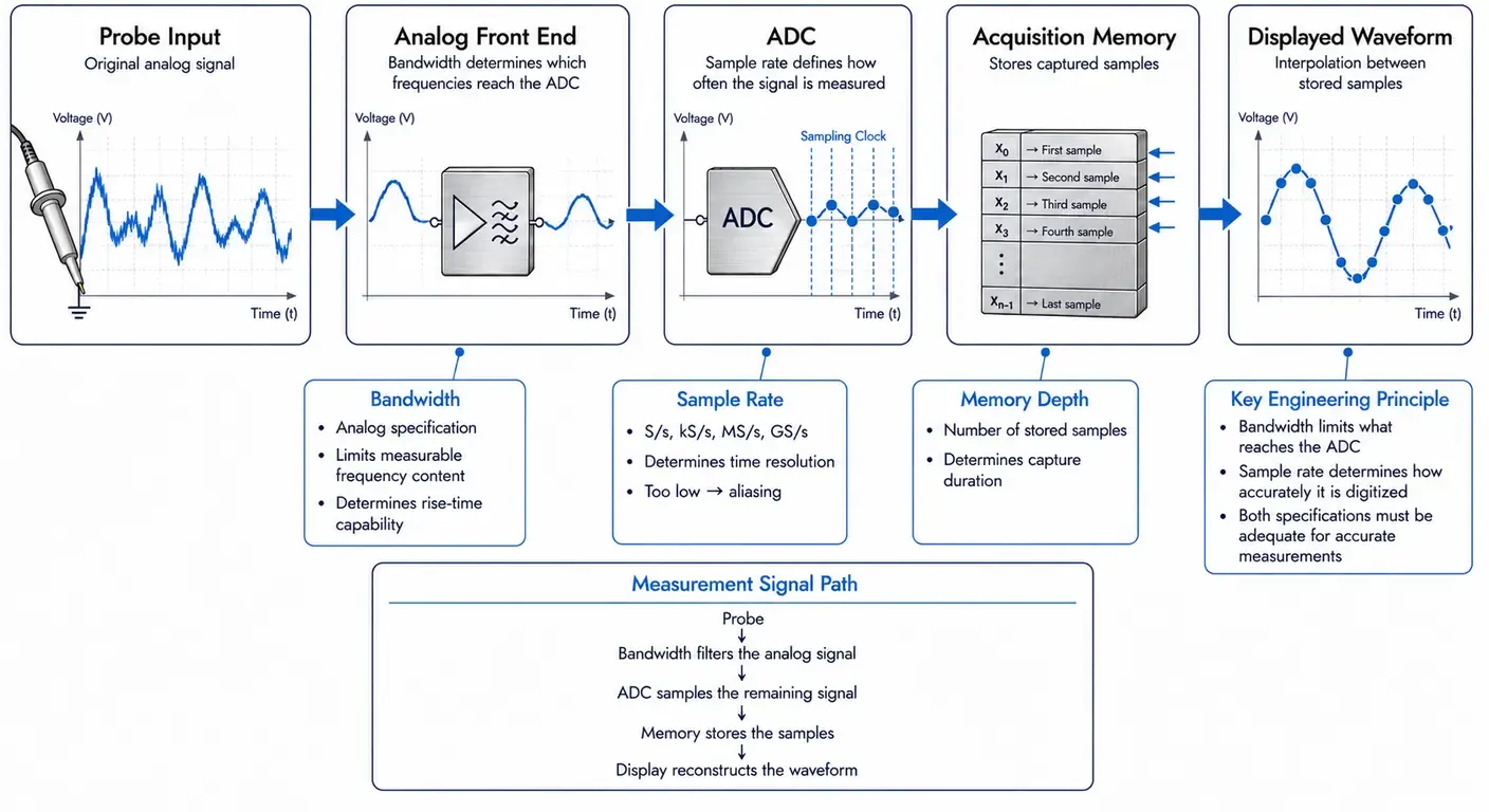
Bandwidth is an analog property of the instrument front end. It is normally defined as the frequency at which the displayed amplitude has fallen by 3 dB, and it describes the highest frequency the instrument can measure with acceptable amplitude accuracy. Sample rate is a digital property describing how often the conditioned signal is measured.
A high sample rate behind a limited front end does not extend measurement capability. The high-frequency content has already been attenuated before it reaches the ADC, and sampling it more often does not restore it. Both specifications must be adequate for the signal under test. Our guide to oscilloscope bandwidth covers the analog side of that combination in depth.
Bandwidth also determines the fastest edge an instrument can display. Rise time is commonly estimated as a constant divided by the bandwidth, where the constant is approximately 0.35 for instruments with a Gaussian-like response and closer to 0.4 or 0.45 for the maximally flat responses used in many higher-bandwidth models. This approximation depends on the instrument response shape and should not replace the rise-time specification provided by the manufacturer. Manufacturers state the applicable figure individually, and it should be taken from the datasheet rather than assumed.
Sample Rate vs Resolution
Resolution describes amplitude rather than time. It is set by the bit depth of the ADC and determines how many discrete levels are available to represent the input range. An 8-bit converter provides 256 levels, so across a 1 V full-scale range each code represents roughly 3.9 mV. A 12-bit converter provides 4096 levels over the same range.
There is a design trade-off between the two specifications. Very fast converters typically offer lower bit depths, while high-resolution converters typically run slower. This is why general-purpose oscilloscopes have traditionally used 8-bit ADCs at very high sample rates, while precision DAQ hardware uses 16-bit or 24-bit converters at far lower rates.
Effective number of bits, or ENOB, is usually the more informative figure. ENOB expresses the resolution actually achieved once noise and distortion in the complete signal path are accounted for, and it degrades with input frequency. A nominally 12-bit instrument may deliver considerably fewer effective bits at the top of its bandwidth, which is why ENOB is normally specified at a stated frequency.
Sample Rate vs Record Length
Record length, also called memory depth, is the number of samples that can be stored in a single acquisition. It defines how much data an instrument can hold, while sample rate defines how quickly that memory is consumed.
The practical consequence is that deep memory is what allows a high sample rate to be maintained over a useful observation window. Without it, capturing a long event forces the instrument to reduce its sample rate, and fine detail is lost even though the instrument is nominally capable of resolving it.
Common Sample Rate Mistakes
Choosing Maximum Sample Rate Without Context
Selecting the highest available sample rate is not automatically the right decision. Higher rates increase data volume, which consumes memory faster and shortens the capture window for a given record length. Large data sets are slower to transfer, process and store, and in continuous acquisition applications the storage requirement grows linearly with rate and channel count. Instrument cost also rises steeply with sample rate.
The appropriate value is the one that satisfies the measurement requirement with reasonable margin, not the largest number on the datasheet.
Ignoring Instrument Bandwidth
A high sample rate cannot recover information that the analog front end has already attenuated. Sampling a 500 MHz signal at 5 GS/s through a 100 MHz front end produces a large quantity of data describing a signal that has been substantially filtered before conversion.
Probes are part of this path and are frequently the limiting element. A high-bandwidth oscilloscope used with a general-purpose passive probe, or with a long ground lead, will produce results constrained by the probe and its ground return, regardless of the instrument specification. The probe bandwidth, its loading on the circuit and the connection method all belong in the measurement budget.
Confusing Sample Rate With Accuracy
Sample rate describes temporal resolution. It says nothing about how accurate the recorded amplitude values are. Measurement quality is the combined result of bandwidth, sample rate, resolution, noise floor, timebase stability, calibration state and probing technique.
An instrument specified at a very high sample rate but with a noisy front end and an unsuitable probe will produce worse results than a more modest instrument used correctly.
Frequently Asked Questions About Sample Rate
What is a good sample rate for an oscilloscope?
There is no single correct value, because the requirement follows the signal rather than the instrument. Start from the highest frequency content that must be captured, including harmonics and edge rates, and apply substantial margin above the Nyquist minimum. Oscilloscope manufacturers and application notes often recommend sample rates several times higher than the bandwidth requirement, with the appropriate factor depending on the interpolation method and the type of measurement. Then verify the rate that applies when all required channels are active, since interleaved architectures reduce the per-channel figure.
Is a higher sample rate always better?
No. A higher sample rate improves temporal detail, but it also consumes acquisition memory faster, shortens the capture window for a given record length, increases data volume and raises instrument cost. It also cannot compensate for insufficient bandwidth or inadequate resolution. The objective is sufficient margin above the measurement requirement, not the highest available figure.
How do you calculate sample rate?
Begin with the highest frequency component present in the signal, not simply the frequency of interest. The Nyquist criterion defines a minimum sample rate of twice that value as an absolute theoretical limit, while practical measurements require considerably more margin, particularly for pulses and fast edges. Then verify the result against the available memory depth: capture time equals memory depth divided by sample rate, so the chosen rate must still allow the required observation window.
What sample rate do I need for digital signals?
The clock frequency is rarely the limiting factor. Rise and fall times determine the highest frequency content in a digital signal, so a moderate clock rate with very fast edges can demand far more bandwidth and sample rate than the clock frequency suggests. Signal complexity also matters: measuring propagation delays, characterising overshoot or capturing narrow glitches all require more samples per edge than simply confirming that a signal is toggling.
What is the difference between sample rate and bandwidth?
Bandwidth is an analog characteristic of the instrument front end and defines the highest frequency it can measure with acceptable amplitude accuracy. Sample rate is a digital characteristic and defines how often the conditioned signal is converted. Bandwidth determines what reaches the ADC, and sample rate determines how finely it is resolved in time. Neither specification compensates for a deficiency in the other.
Sample rate is best understood as one parameter within a coordinated set. It defines how finely an instrument resolves time, while bandwidth defines what reaches the converter, resolution defines how finely amplitude is quantified, and memory depth defines how long the acquisition can run. Engineers who evaluate these specifications together, under the conditions stated in the datasheet and against the actual characteristics of the signal under test, consistently obtain more reliable measurements than those who compare a single headline figure across product pages.
Related articles
Electronics18 min read
Function Generator vs Arbitrary Waveform Generator: What You Are Buying
Three names, two architectures: how DDS and point-by-point playback differ, what the labels hide, and how to read the architecture off a datasheet.
Electronics23 min read
How to Choose a Signal Generator: Getting the Signal You Asked For
How to turn a required stimulus into datasheet requirements: the load the instrument assumes, bandwidth against sample rate, reconstruction and vertical resolution.
Electronics22 min read
How to Choose a Multimeter: A Specification-Led Buying Guide
Choose a multimeter by the errors it introduces: burden voltage, input loading, AC bandwidth, safety category and accuracy on the reading you actually take.
Electronics16 min read
How to Use a Thermal Camera: Getting Readings You Can Trust
A thermal camera always shows a number. Learn the checks — emissivity, reflected temperature, focus and spot size — that decide whether it is a measurement.