Oscilloscope Probe Guide: Types, Selection, Compensation, and Best Practices
A complete oscilloscope probe guide covering probe types, attenuation, bandwidth, loading, compensation, grounding and safety ratings for accurate measurements.
By YDT EditorialUpdated 35 min read
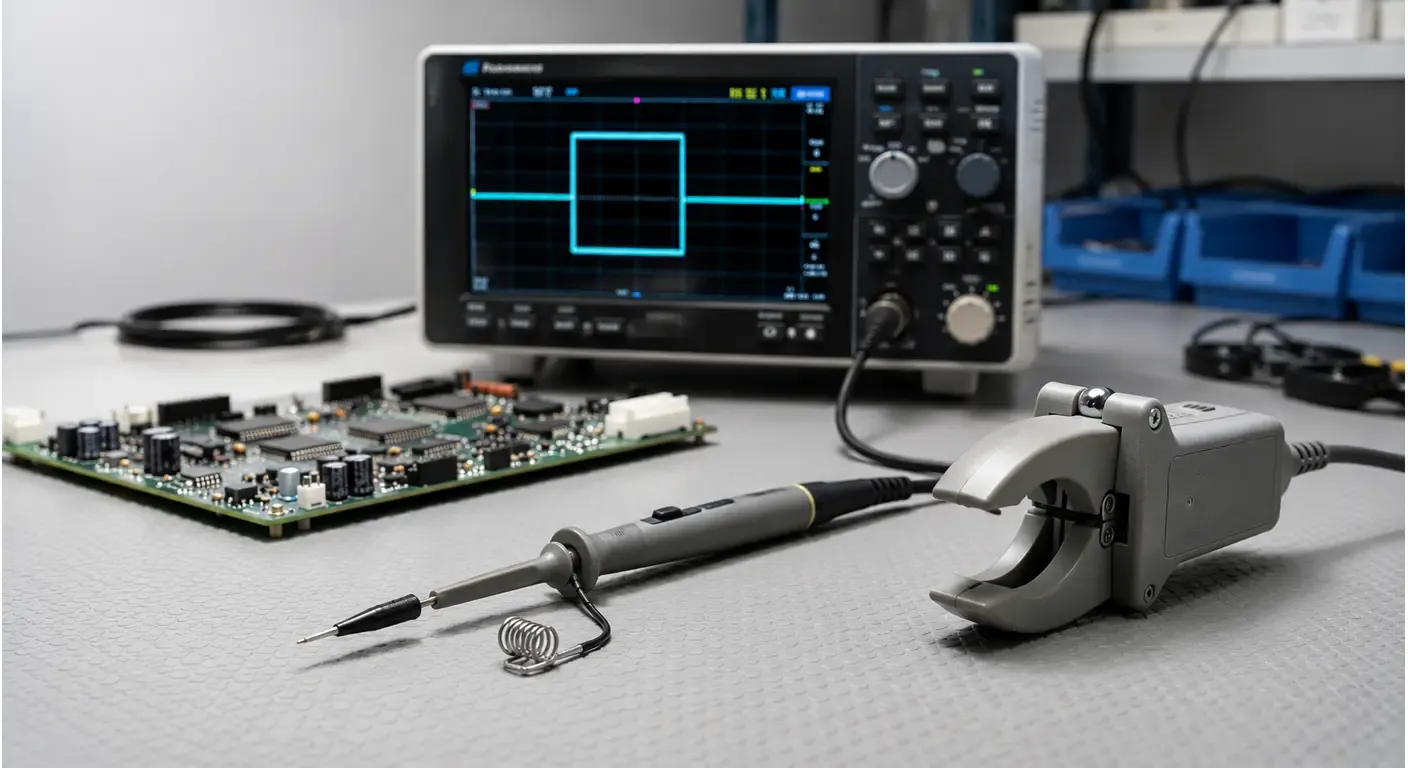
A large share of the measurement errors that engineers attribute to the oscilloscope originate in the first ten centimeters of the signal path.
An edge that overshoots on screen but not in the circuit. A ripple measurement that changes value when the probe is moved. An oscillator that stops oscillating the moment it is probed. In each case the instrument is reporting exactly what arrives at its input — the problem is what happened between the circuit node and that input.
That path is the probe. It is the only part of the measurement system that physically touches the circuit under test, and it is frequently selected by default rather than by decision.
This oscilloscope probe guide covers what probes do to a signal, how the main probe families differ, and how attenuation, compensation, grounding and safety ratings determine whether a measurement can be trusted. It is one part of a larger discipline — our complete Test & Measurement guide covers the rest of the instruments on a bench and where probing fits among them.
Introduction to Oscilloscope Probes
What is an oscilloscope probe?
An oscilloscope probe is a device that connects a circuit node to an oscilloscope input while controlling how much the connection disturbs the circuit and how faithfully the signal survives the journey.
The definition matters because the intuitive alternative — a piece of wire — fails quickly. A wire has inductance, forms a loop with its return path, and presents the oscilloscope’s full input capacitance directly to the node under test. At audio frequencies this is tolerable. At the edge rates found in most modern digital and switching designs, it is not.
A probe is therefore a designed network. In a typical 10X passive probe:
- a resistor and a trimmer capacitor at the tip form the first half of a compensated divider;
- a specially constructed low-capacitance cable carries the attenuated signal;
- a compensation box terminating in a BNC connector completes the divider against the oscilloscope’s own input impedance.
Each element exists to solve a specific problem, and each imposes a specific cost.
Why probe selection matters
An oscilloscope’s specifications are measured at its input connector. Everything ahead of that connector is the responsibility of the probe, and the probe can consume a significant fraction of the performance the instrument was purchased for.
A 1 GHz oscilloscope used with a 500 MHz probe forms a measurement system of approximately 450 MHz. A 200 MHz probe on a 200 MHz oscilloscope yields roughly 140 MHz of usable bandwidth. The instrument’s front panel still displays its original specification; the signal path no longer supports it.
Selection also determines what is measurable at all. A ground-referenced passive probe cannot safely measure a high-side gate drive. A voltage probe cannot measure inductor current. A 10X probe measuring 5 mV of power rail ripple spends most of its dynamic range delivering little more than noise.
How probes influence measurement accuracy
Probes affect measurements through three mechanisms, and it is worth separating them because the remedies differ.
Loading changes the circuit. The probe’s resistance, capacitance and ground-loop inductance appear in parallel with the node under test, altering the signal that exists there.
Band limiting changes the signal in transit. The probe has a finite frequency response that combines with the oscilloscope’s own, and the combination sets the achievable measurement uncertainty.
Coupling adds signal that was never there. Ground loops, long ground leads and unshielded tip extensions pick up radiated energy from nearby switching nodes.
How Oscilloscope Probes Work
Signal transmission fundamentals
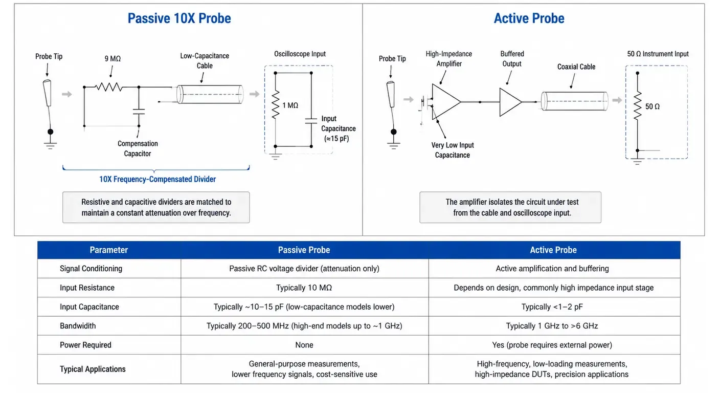
A passive probe is best understood as a frequency-compensated voltage divider that happens to have a cable in the middle.
At the tip, a series resistance sets the division ratio against the oscilloscope’s 1 MΩ input resistance. For a 10X probe this is 9 MΩ at the tip, giving 9 MΩ + 1 MΩ divided by 1 MΩ, or a 10:1 ratio. The oscilloscope reads one tenth of the applied voltage and multiplies the displayed values back up.
Resistance alone would produce a working divider at DC and a low-pass filter at everything else. The cable and the oscilloscope front end contribute capacitance — instrument input capacitance commonly falls between about 6 pF and 35 pF, with higher-bandwidth instruments at the lower end, and the probe cable adds more. Combined with 1 MΩ, that capacitance would place a pole in the low kilohertz region.
The solution is to add a matching capacitance across the tip resistor so that the divider divides capacitively by the same ratio it divides resistively. When the two RC time constants are equal, the division ratio becomes largely independent of frequency.
Setting that equality is what probe compensation does.
Active probes work differently. An amplifier is placed at the tip itself, so the circuit under test sees only the amplifier’s input, and the cable carries a buffered low-impedance signal into a 50 Ω instrument input.
Probe impedance
Probe impedance is quoted as a resistance in parallel with a capacitance, typically written as something like 10 MΩ ‖ 10 pF. Both numbers matter, but they matter at different frequencies.
The resistance dominates at DC and low frequencies. The capacitance dominates as soon as its reactance falls below the resistance, and it falls quickly:
Xc = 1 / (2πfC)
For 10 pF, the reactance is about 159 kΩ at 100 kHz, about 1.6 kΩ at 10 MHz, and about 159 Ω at 100 MHz. The 10 MΩ headline figure has become largely irrelevant well before the oscilloscope reaches its bandwidth limit.
Approximate impedance of common probe tip capacitances versus frequency
- 10 pF at 1 MHz
- ≈ 16 kΩ
- 10 pF at 100 MHz
- ≈ 159 Ω
- 3.9 pF at 100 MHz
- ≈ 408 Ω
- 1 pF at 100 MHz
- ≈ 1.6 kΩ
- 1 pF at 1 GHz
- ≈ 159 Ω
Oscilloscope input impedance itself comes in two standard forms, and the probe must match the one selected. A 1 MΩ input is intended for high-impedance passive probes and for most active probe interfaces; a 50 Ω input is intended for direct coaxial connection and for transmission-line probes, and offers far less tolerance to the voltages a 1 MΩ input handles routinely.
The practical consequence is that input capacitance, rather than input resistance, is the specification that separates probes for high-speed work. A probe with 1 pF at the tip presents ten times the impedance of a 10 pF probe at every frequency.
Probe loading effects
Loading is the change the probe causes in the circuit it is measuring. It is easiest to reason about by asking what the probe adds in parallel with the node.
Resistive loading is usually negligible for high-impedance probes. A 10 MΩ probe across a 5 V node driven from a 1 kΩ source changes the DC level by well under a millivolt. The exceptions are high-impedance sensor nodes, bias networks and long-time-constant RC circuits, where even 10 MΩ can shift a level or slow a settling time.
Capacitive loading is usually where the real damage occurs. Adding 10 pF to a node driven through 1 kΩ creates a 10 ns time constant, corresponding to roughly a 16 MHz pole. A 5 ns edge arriving at that node will be visibly slowed — and it will be genuinely slowed in the circuit, not merely on the display.
The effect scales with source impedance:
| Source impedance | Added time constant with 10 pF | Practical consequence |
|---|---|---|
| 20 Ω (buffered driver) | 0.2 ns | Negligible for most digital work |
| 220 Ω (series-terminated line) | 2.2 ns | Visible on edges faster than about 5 ns |
| 1 kΩ (pull-up, sense node) | 10 ns | Slows edges and can shift logic timing |
| 100 kΩ (bias network, sensor) | 1 µs | Circuit behavior changes outright |
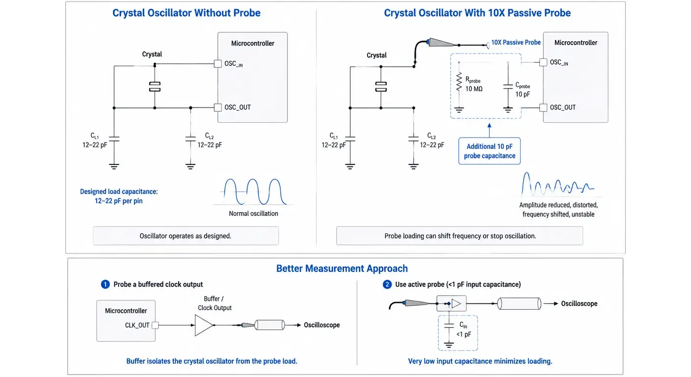
Worked example — the crystal oscillator. A 16 MHz crystal driven by a microcontroller’s internal inverter typically sees a load capacitance budget of 12 pF to 22 pF per pin, deliberately balanced by the designer. Touching the drive pin with a 10 pF passive probe roughly doubles one side of that budget. The oscillator may shift frequency measurably or stop entirely, and the engineer concludes the crystal is faulty. A more reliable approach is to probe the buffered clock output instead, or to use an active probe whose tip capacitance is below 1 pF.
Bandwidth limitations
Probe bandwidth is specified with a defined tip accessory and a short ground connection, measured into the intended instrument input. Both conditions are part of the specification, not fine print — the same probe fitted with a six-inch ground lead will not generally meet its published figure.
Probe and oscilloscope bandwidths combine approximately as a root-sum-square of their rise times, which for Gaussian-response systems gives:
1 / BW_system² ≈ 1 / BW_scope² + 1 / BW_probe²
| Oscilloscope bandwidth | Probe bandwidth | Approximate system bandwidth |
|---|---|---|
| 200 MHz | 200 MHz | 141 MHz |
| 200 MHz | 500 MHz | 186 MHz |
| 500 MHz | 500 MHz | 354 MHz |
| 1 GHz | 500 MHz | 447 MHz |
| 1 GHz | 1.5 GHz | 832 MHz |
Two equal elements cost roughly 30% of the headline figure. A faster element contributes little once it is well ahead of the slower one, which is why probe bandwidth is generally kept at or above instrument bandwidth and the pair treated as a system.
System bandwidth then determines amplitude uncertainty. For an instrument with a Gaussian response, the error at the highest frequency of interest follows from the ratio between system bandwidth and that frequency:
Approximate amplitude error versus the ratio of system bandwidth to signal frequency (Gaussian response)
- BW = 1 × f
- ≈ 29% low (the −3 dB point)
- BW = 2 × f
- ≈ 8% low
- BW = 3 × f
- ≈ 4% low
- BW = 5 × f
- ≈ 1.4% low
The same limitation expressed in the time domain is rise time, related to bandwidth by BW × tr ≈ 0.35 for Gaussian instruments. Because probe and oscilloscope rise times add in quadrature with the signal’s own, a measurement system whose rise time equals the signal’s rise time reports an edge about 41% slower than reality. Our article on oscilloscope bandwidth covers how much system bandwidth a given signal actually requires.
Types of Oscilloscope Probes
Six probe families cover the majority of bench and field work. The table below summarizes where each belongs before the sections that follow examine them individually.
| Probe family | Measures | Typical loading | Typical bandwidth range | Reference to instrument |
|---|---|---|---|---|
| Passive high-impedance | Voltage | 10 MΩ ‖ 4–15 pF | DC to 100 MHz–1 GHz | Earth-referenced |
| Active single-ended | Voltage | 100 kΩ–1 MΩ ‖ under 1–2 pF | DC to several GHz | Earth-referenced |
| Differential | Voltage between two nodes | High, matched inputs | DC to hundreds of MHz | Floating within common-mode limit |
| Current | Current | Insertion impedance | AC-only or DC to tens of MHz | Galvanically isolated |
| High-voltage | Voltage | 50–100 MΩ ‖ a few pF | DC to tens of MHz | Earth-referenced or differential |
| Transmission-line | Voltage | Few hundred Ω resistive | To multiple GHz | 50 Ω input required |
Passive probes
Passive probes contain no active components and require no power. The 10X high-impedance passive probe is the industry’s default accessory, supplied with almost every bench oscilloscope sold.
Typical characteristics are 10 MΩ input resistance and tip capacitance between roughly 9 pF and 15 pF, with bandwidths that historically topped out around 500 MHz. Low-capacitance designs have pushed this further; probes with tip capacitance near 4 pF and bandwidths of 1 GHz are available, though they are generally matched to specific instrument families.
Passive probes are rugged, inexpensive, tolerant of abuse, and offer wide dynamic range — commonly 300 V CAT II for general-purpose models. They are usually the appropriate tool for supply rails, logic-level signals, control lines and routine debugging.
Active probes
Active probes place a high-impedance amplifier at the probe tip. Because the circuit sees only the amplifier input, tip capacitance can be brought below 1 pF, and bandwidths extend into the multi-gigahertz region.
The trade-offs are substantial:
- Dynamic range is limited, often to a window of roughly ±10 V or less around an adjustable offset.
- The probes require power and scale-factor communication through a proprietary instrument interface.
- They cost considerably more than passive probes.
- They are physically fragile; an overvoltage event at the tip can destroy the amplifier.
Active probes are chosen when loading or bandwidth would otherwise dominate the measurement: high-speed serial links, fast clock edges, and nodes whose impedance is high enough that 10 pF would alter the result.
Differential probes
A differential probe measures the voltage between two points, neither of which needs to be at ground potential. Two matched inputs feed a differential amplifier, and the output represents the difference between them.
Two specifications govern their use.
Common-mode voltage range defines how far the pair of inputs may float above earth before the amplifier saturates or the probe is damaged. A probe with a 1000 V common-mode rating and a 100 V differential range can measure a 50 V gate drive sitting 600 V above ground; the same probe would not be suitable for an 800 V traction inverter.
Common-mode rejection ratio (CMRR) describes how effectively the probe ignores the voltage common to both inputs. CMRR degrades with frequency — a probe offering 80 dB at DC may offer only 30 dB at 1 MHz — so the specification should be read at the frequency of interest rather than at DC.
Differential probes are generally required wherever the node of interest is not referenced to earth: high-side gate drive signals, motor drive phase voltages, current sense resistors sitting above ground, and offline switch-mode supply primaries. They are covered in detail in our differential probe guide.
Current probes
Current probes measure current without breaking the circuit, by clamping around the conductor.
AC-only current probes are passive current transformers. They are simple and can reach high bandwidths, but they cannot measure DC and will saturate if significant DC flows through the conductor.
AC/DC current probes combine a current transformer with a Hall effect sensor, splitting the measurement between the two and summing the results. They measure from DC upward and require power, degaussing and zeroing before use.
Rogowski coils use an air-cored winding and an integrator. They handle very large currents and awkward geometries, but respond only to changing current.
Every current probe adds insertion impedance to the circuit, and each has a peak current limit beyond which the core saturates and readings become unreliable. Because current probes introduce a propagation delay that differs from that of a voltage probe, any measurement combining the two — switching loss, for instance — requires deskew before the result carries meaning. See our current probe guide for selection detail.
High-voltage probes
High-voltage probes extend the measurable range through higher attenuation ratios — typically 100X or 1000X — combined with physical construction that provides the necessary creepage and clearance distances.
They exist in single-ended and differential forms. A single-ended high-voltage probe still references the oscilloscope’s earthed ground and carries all the constraints that implies. A high-voltage differential probe does not, which is why it is the usual tool for power electronics work. Our high-voltage probe guide covers the distinction.
Special-purpose probes
Several other probe families address specific measurement problems.
Transmission-line probes present a resistive tip impedance of a few hundred ohms into a 50 Ω instrument input. They offer excellent high-frequency fidelity with very low capacitance, at the cost of significant resistive loading.
Logic probes connect digital channels on a mixed-signal oscilloscope, presenting a threshold comparator rather than an analog front end.
Near-field probes sense magnetic or electric field rather than voltage, and are used for EMC pre-compliance work and for locating radiating structures.
Optically isolated probes provide very high common-mode rejection and isolation voltage for measurements where a conventional differential probe’s CMRR is insufficient.
Passive vs Active Probes
Operating principles
The distinction is structural.
A passive probe divides the signal down and sends the result along a cable to the oscilloscope, which means the oscilloscope’s input capacitance forms part of the network and the circuit sees the whole assembly.
An active probe amplifies at the tip, isolating the circuit from everything downstream. The trade is that the circuit now faces a semiconductor input rather than a resistor, with the range and fragility limits that implies.
Advantages, limitations and typical applications
| Characteristic | Passive probe (10X) | Active probe |
|---|---|---|
| Tip capacitance | Typically 9–15 pF, low-capacitance types near 4 pF | Typically under 1–2 pF |
| Bandwidth | Commonly to 500 MHz, some to 1 GHz | Multiple GHz available |
| Dynamic range | Wide, often 300 V CAT II | Narrow, often within ±10 V of offset |
| Power required | None | Yes, from instrument |
| Robustness | High | Low; overvoltage damages the tip amplifier |
| Noise contribution | None added | Amplifier noise adds to the measurement |
| Relative cost | Low | High |
| Typical use | Rails, logic, control signals, general debugging | High-speed edges, serial links, high-impedance nodes |
The comparison explains why most benches hold both. Passive probes handle the bulk of the work and survive contact with things they should not have touched. Active probes are reserved for measurements where a passive probe’s capacitance would change the answer.
Selection criteria
An active probe is generally warranted when at least one of the following is true:
- the signal edge is faster than roughly 1 ns;
- the node impedance is high enough that 10 pF creates a meaningful time constant;
- the required bandwidth exceeds what any passive probe supports.
Otherwise, a good passive probe with a proper ground connection will often outperform a poorly applied active probe.
Understanding Probe Attenuation
What attenuation means
Probe attenuation is the fixed division ratio applied to the signal before it reaches the oscilloscope. A 10X probe delivers one tenth of the applied voltage; the instrument multiplies its readings by ten to display the true value.
Attenuation is not free. Dividing the signal also divides it relative to the oscilloscope’s own input noise, so higher attenuation generally costs signal-to-noise performance.
| 1X | 10X | 100X | |
|---|---|---|---|
| Tip resistance into 1 MΩ | None | 9 MΩ | 99 MΩ |
| Input capacitance | Typically 50–120 pF | Typically 4–15 pF | A few pF |
| Typical bandwidth | 6–35 MHz | To 500 MHz, some to 1 GHz | Tens of MHz |
| Effect on noise floor | Best | Moderate | Worst |
| Typical voltage range | Low | 300 V CAT II class | kV class |
| Best suited to | Millivolt signals below a few MHz | General-purpose measurement | High-voltage work |
1X probes
A 1X probe passes the signal through unattenuated. The full amplitude reaches the oscilloscope, which is valuable when measuring small signals — a 10 mV ripple measured through a 10X probe arrives at the front end as 1 mV, uncomfortably close to the instrument’s noise floor.
The cost is significant. Without the tip divider network, the probe presents the cable and instrument capacitance almost directly to the circuit, commonly 50 pF to over 100 pF, and bandwidth typically collapses to somewhere between 6 MHz and 35 MHz depending on the design.
1X is best suited to low-frequency, low-amplitude work: audio, sensor outputs, slow control loops, and supply ripple below a few megahertz.
10X probes
The 10X probe is the general-purpose standard. It provides the 10 MΩ ‖ 10 pF characteristic that most oscilloscope inputs are designed around, supports the probe’s full rated bandwidth, and leaves useful dynamic range headroom.
100X probes
Raising the ratio to 100X requires 99 MΩ at the tip against a 1 MΩ instrument input. This extends the usable voltage range considerably and further reduces loading, which is why the ratio is common in high-voltage probes.
The penalty is noise. A 1 V signal arriving at the oscilloscope as 10 mV sits low in the front end’s range, and the displayed noise scales up by the same factor of 100.
Choosing the correct attenuation
| Situation | Preferred attenuation | Reason |
|---|---|---|
| General digital and analog debugging | 10X | Best balance of loading, bandwidth and dynamic range |
| Millivolt-level ripple or noise below a few MHz | 1X | Preserves signal-to-noise ratio where bandwidth is not the constraint |
| Signals above the instrument’s 10X input range | 100X | Extends range and reduces loading |
| Any measurement above 50 MHz | 10X or lower-capacitance active | 1X bandwidth is insufficient |
Worked example — SMPS output ripple. A 3.3 V buck converter specified for 20 mV peak-to-peak ripple presents two competing problems. Through a 10X probe, 20 mV becomes 2 mV at the front end, largely buried in noise. Through a 1X probe the amplitude is preserved, but the probe’s limited bandwidth removes the switching spikes that often dominate the true figure. A common resolution is a low-attenuation measurement taken directly across the output capacitor with a ground spring, with the oscilloscope’s bandwidth limit set deliberately to the value the specification calls for rather than left wherever it happened to be.
Probe Compensation
Why compensation is necessary
The passive probe divider divides equally at all frequencies only when the tip RC product matches the instrument-side RC product. The resistances are fixed and accurate. The capacitances are not: instrument input capacitance varies between models, cable capacitance varies between units, and the total must be trimmed for each pairing.
That trimming is probe compensation. It is not a calibration of the oscilloscope, and it does not improve the probe’s high-frequency response; it aligns the low-frequency behavior of the divider with its high-frequency behavior so that a square wave stays square.
Three operations are routinely confused, and separating them prevents a great deal of wasted bench time:
| Operation | What it corrects | When it is performed |
|---|---|---|
| Compensation | Low-frequency divider mismatch between probe and instrument input | Each time a passive probe meets a new channel or instrument |
| Probe calibration | Gain and offset error of an active or current probe | Periodically, and after temperature change, using the instrument’s routine |
| Deskew | Propagation delay differences between channels or probe types | Before any multi-channel timing or power measurement |
Our dedicated article on oscilloscope probe compensation walks through the procedure in more depth.
Compensation procedure
- Connect the probe to the oscilloscope channel it will be used on and set that channel’s attenuation to match the probe.
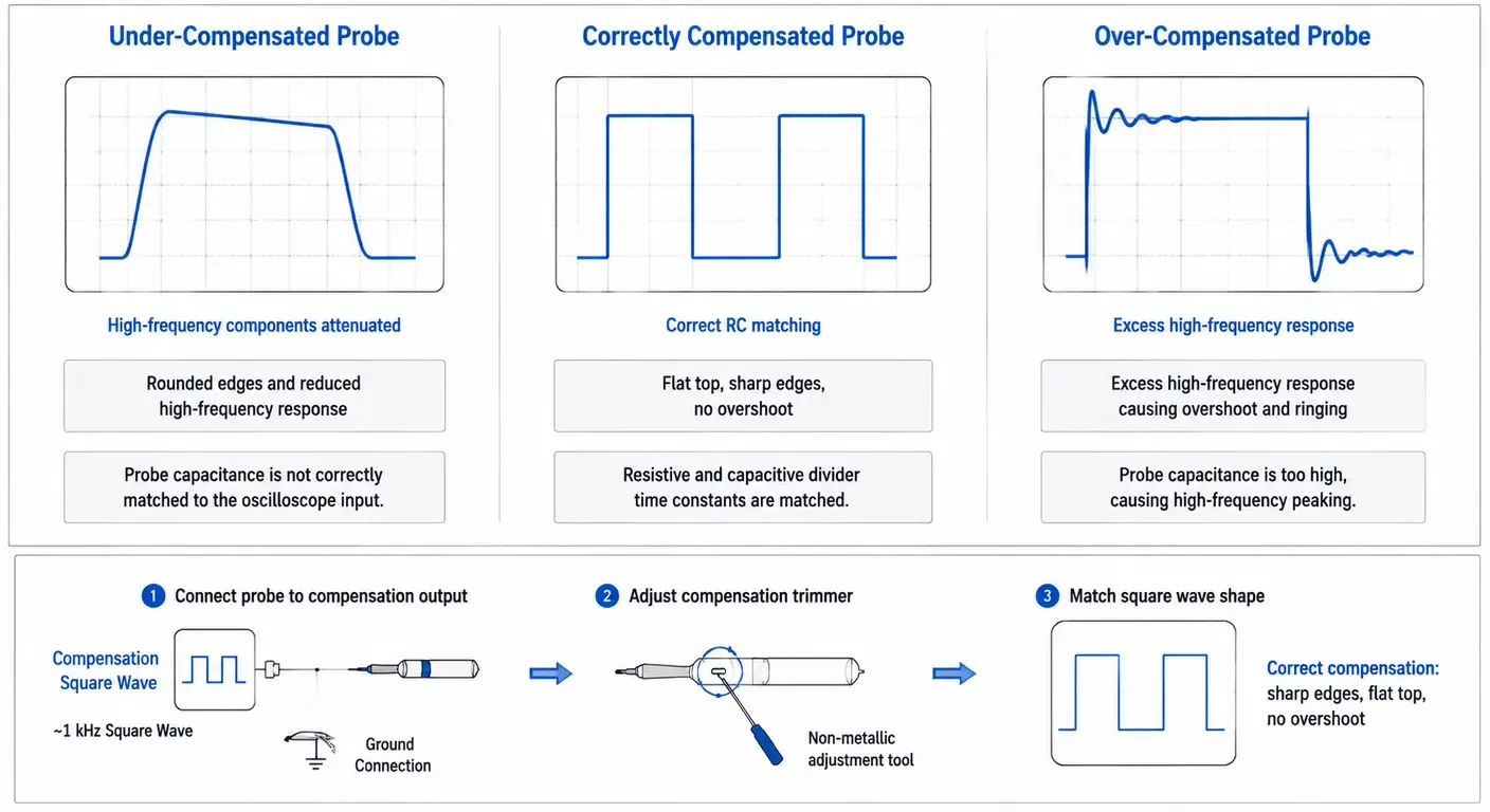
- Connect the probe tip to the instrument’s probe compensation output — a compensation square wave of a few volts at around 1 kHz — and attach the ground clip to the adjacent ground terminal.
- Adjust the timebase and vertical scale so that two or three cycles fill most of the display.
- Using the non-metallic adjustment tool supplied with the probe, turn the compensation trimmer until the top of the square wave is flat, with square corners and no overshoot or rounding.
- Verify by expanding the timebase around a single edge.
Some high-bandwidth passive probes provide additional adjustments intended to be set against a fast-edge source rather than the 1 kHz output, and certain probe and instrument combinations perform the entire process automatically.
Recognizing under-compensation
Under-compensation means the tip capacitance is too small relative to the instrument side. High-frequency content is attenuated more than low-frequency content, so edges arrive rounded and the flat top slopes upward toward its final value.
Amplitude measurements taken on fast pulses will read low, which understates overshoot and overstates rise time margin at the same time.
Recognizing over-compensation
Over-compensation is the opposite condition. High-frequency content is emphasized, producing a peaked leading edge and a top that decays downward toward the correct level.
This is generally the more troublesome error, because it manufactures overshoot that does not exist in the circuit and invites engineers to fix problems that are not there.
Properly compensated waveform
A correctly compensated probe reproduces the compensation signal with a flat top, a flat bottom, and a corner that is sharp without ringing.
Compensation should be rechecked whenever a probe is moved to a different channel or instrument, after significant temperature change, and periodically as part of routine bench discipline.
Grounding and Measurement Quality
Ground leads and inductance
Every probe needs a return path, and that return path has inductance. Small-gauge wire contributes roughly 20 nH per inch, so a standard six-inch alligator-clip ground lead contributes on the order of 120 nH.
That inductance is in series with the measurement, and it forms a resonant circuit with the probe’s tip capacitance:
f = 1 / (2π√(LC))
With 120 nH and 10 pF, the resonance sits near 145 MHz. Any signal with edge content in that region will tend to excite it.
Approximate ground-loop resonance with a 10 pF probe tip capacitance
- 150 mm alligator lead, ≈ 120 nH
- ≈ 145 MHz
- 75 mm lead, ≈ 60 nH
- ≈ 205 MHz
- Short ground blade, ≈ 20 nH
- ≈ 356 MHz
- Ground spring, ≈ 5 nH
- ≈ 712 MHz
Ground springs
The ground spring is a short coil that clips over the probe barrel and contacts ground within a few millimeters of the tip. By collapsing the loop area and shortening the return path, it reduces inductance by more than an order of magnitude and moves the resonance well above the frequencies of interest.
It is among the most effective probing accessories available, and one of the least used. The wider family of probe tip accessories — micro-hooks, browser tips, spring-loaded pins, ground blades and solder-in leads — exists for the same reason: to shorten both the signal and return paths at the point of contact.
Reducing ringing
Ringing on a captured edge is best treated as a hypothesis rather than a finding.
Before investigating the circuit, shorten the ground path and repeat the measurement. If the ringing frequency changes, it belonged to the probe. If both amplitude and frequency remain identical, the circuit is genuinely ringing and the investigation can proceed — a distinction explored further in our article on signal integrity basics.
Worked example — debugging a SPI bus. A 20 MHz SPI clock with 2 ns edges contains meaningful spectral content beyond 150 MHz. Probed with four passive probes on standard alligator leads, the clock shows 40% overshoot and the chip select line appears to glitch. Refitting ground springs and grounding each probe at the return pin of the target device removes both artifacts.
The overshoot was ground-loop resonance near 145 MHz; the apparent glitch was crosstalk picked up by the ground loops themselves. Only after that correction is it worth deskewing the channels and measuring setup and hold times.
Minimizing measurement errors
A few practices account for most of the improvement available:
- Ground as close to the signal as the board layout permits, ideally at the return pin of the device being measured.
- Use the shortest ground accessory that will physically reach.
- Avoid grounding one probe and daisy-chaining others to it; each probe needs its own local return.
- Deskew channels before comparing timing across probes of different types or cable lengths.
- Check for pickup by touching the probe tip to its own ground connection. A flat trace suggests the loop is quiet; anything else is being received rather than measured.
Probe Safety
Voltage ratings
A probe’s voltage rating defines the maximum it can safely handle, and it is frequently specified as a peak value rather than an RMS value.
A probe rated 300 V CAT II is not rated for 300 V RMS on every waveform — the derating curve, which reduces permissible voltage as frequency rises, is part of the specification and appears in the datasheet. On a PWM waveform with fast edges, the applicable limit can be a fraction of the headline number.
CAT safety ratings
Measurement categories describe transient withstand capability rather than steady-state voltage. They exist because the energy available behind a circuit varies enormously with its position in an installation: a transient on a distribution panel carries far more energy than the same voltage appearing at a plug-in appliance.
The categories are defined in IEC 61010-1, and the specific safety requirements for hand-held and hand-manipulated probe assemblies are set out in IEC 61010-031, whose second edition was published in 2015 and replaced the 2002 first edition.
| Category | Applies to | Representative measurements |
|---|---|---|
| Not rated for CAT II/III/IV | Circuits isolated from mains | Bench supplies, battery-powered boards, signal electronics |
| CAT II | Circuits connected to standard outlets and plug-in loads | Appliance internals, offline SMPS on a bench outlet |
| CAT III | Distribution wiring and permanently installed equipment | Motor drives, distribution boards, fixed machinery |
| CAT IV | Origin of the installation, service entrance, outdoor conductors | Utility connections, main panels, overhead supply |
One point of terminology is worth knowing, because older probes and older documents still use it. In the current probe standard, the designation “measurement category I” has been replaced by the statement that a probe is not rated for measurements within categories II, III or IV. In practice this means an unrated probe belongs only on circuits isolated from mains.
Ground-referenced measurements
The ground connection on a standard passive probe is bonded through the oscilloscope chassis to protective earth. Connecting that clip to a node that is not at earth potential creates a short circuit through the instrument, and the fault current flows through the probe cable, the oscilloscope and the mains earth conductor.
The consequences range from a destroyed probe to a destroyed instrument to injury.
Defeating the oscilloscope’s earth connection to work around this is not an acceptable substitute: it leaves every exposed metal surface of the instrument, including all BNC shells, floating at the potential of whatever the ground clip is touching. Since the BNC outer conductors of all channels are commonly bonded together, a single misplaced ground clip also ties every other probe’s reference to the same node.
When differential probes are required
Use a differential probe whenever neither measurement point can be safely connected to earth. Typical cases include:
- the primary side of an offline power supply;
- motor drive and inverter phase outputs;
- high-side gate drive signals in a half-bridge;
- current sense resistors located above ground;
- any measurement across a component in a floating circuit.
Worked example — an industrial motor drive. Measuring the gate-source voltage of the upper IGBT in a 400 V three-phase inverter means measuring a 15 V signal riding on a node that swings the full DC link voltage in tens of nanoseconds. A passive probe would short the phase node to earth on contact. The appropriate instrument is a differential probe whose common-mode range exceeds the DC link voltage with margin, and whose CMRR at the switching edge rate is high enough that the 400 V common-mode step does not swamp the 15 V differential signal.
Selecting the Right Probe
Probe selection is a sequence of constraints rather than a preference. The order matters: safety constraints eliminate options outright, electrical constraints narrow what remains, and only then does convenience decide.
Bandwidth requirements
Work from the fastest edge in the system rather than the clock frequency. A 1 MHz PWM signal with 5 ns edges is a high-bandwidth measurement; a 50 MHz sine wave is not.
Convert edge rate to a knee frequency using f_knee ≈ 0.5 / tr for a 10% to 90% rise time, or 0.4 / tr for 20% to 80%, then require system bandwidth of 1.0 to 1.9 times that value. Keep probe bandwidth at or above the oscilloscope’s so the probe is not the limiting element, and where the two are close, calculate the system figure rather than assuming the higher number applies. The relationship between edge rate and required bandwidth is covered in our article on rise time and edge measurement.
Voltage range
Establish the maximum voltage the probe will encounter, including transients and fault conditions rather than only the nominal operating level.
Confirm three things in the datasheet: the absolute maximum input, the derating curve at the frequencies involved, and the measurement category appropriate to where the circuit sits in the installation. For differential and high-voltage probes, add the common-mode voltage rating to that list.
Input impedance
Compare the probe’s tip capacitance against the source impedance of the node.
As a working check, multiply the two: a 1 kΩ source with a 10 pF probe gives 10 ns, which will visibly affect any edge faster than about 30 ns. If the product approaches the timescale of interest, a lower-capacitance probe is required — or the measurement should move to a lower-impedance point in the circuit.
Measurement environment
Physical access constrains probe choice more often than engineers expect.
Fine-pitch packages need browser tips or solder-in leads. Rotating machinery and enclosed assemblies need clamp-on current probes. Elevated temperature and vibration rule out delicate active probe tips. Field work on live panels rules out anything without the appropriate CAT marking, regardless of its electrical performance.
Application examples
The following decision process reduces most selection problems to a short sequence of questions.
- Is either measurement point at a potential other than earth? If yes, a differential or isolated probe is required. No other consideration overrides this.
- Is the quantity current rather than voltage? If yes, select a current probe, then decide between AC-only and AC/DC by whether a DC component exists.
- Does the circuit sit within a mains installation? If yes, the probe must carry a CAT rating at or above the installation category, at or above the working voltage.
- What is the fastest edge? Convert to a knee frequency and set the required system bandwidth.
- What is the source impedance at the probe point? Multiply by candidate tip capacitance; if the product is comparable to the edge rate, move to a lower-capacitance probe.
- What is the signal amplitude? Small signals favor lower attenuation; large signals force higher attenuation and accept the noise penalty.
- Can the probe physically reach the node? Select tip accessories before assuming the measurement is possible.
                        Voltage or current?
                          |            |
                     voltage        current
                          |            |
        Floating measurement?     DC component present?
            |          |               |         |
           yes         no             yes        no
            |          |               |         |
   Differential   Amplitude?       AC/DC     AC-only
    or isolated       |          current      current
     probe            |           probe        probe
                      |
        ----------------------------
        |             |            |
    above 300 V   under 300 V   millivolts
        |             |            |
  High-voltage   Edge faster    1X or low
     probe        than 1 ns?    attenuation
                   |      |
                  yes     no
                   |      |
              Active   10X passive
probe probe| Application | Typical probe choice | Reasoning |
|---|---|---|
| PCB debugging | 10X passive with ground spring | Adequate bandwidth, robust, low cost, wide dynamic range |
| Embedded systems | 10X passive; low-capacitance passive for fast buses | Most signals are buffered logic; loading matters on high-impedance lines |
| Power electronics | High-voltage differential plus AC/DC current probe | Nodes are floating; current waveforms are essential to the analysis |
| Automotive electronics | Differential probe with appropriate CAT rating; current probe for loads | Chassis reference is unreliable; high-voltage systems demand isolation |
| Industrial maintenance | CAT III or CAT IV rated differential probe | Available transient energy is high; measurements are often on live panels |
| RF testing | Transmission-line probe or direct 50 Ω connection | Impedance control dominates; capacitance must be minimal |
Worked example — automotive electronics. A CAN bus fault on a 12 V vehicle looks like a low-voltage measurement, and engineers routinely probe CANH and CANL against chassis with two passive probes. The result is often misleading, because the fault of interest is differential and the chassis reference carries the voltage drop of every high-current load on the vehicle. A single differential probe across CANH and CANL removes the chassis from the measurement entirely. On a hybrid or electric vehicle the same reasoning becomes a safety requirement rather than an accuracy improvement, since the traction system operates at several hundred volts with no earth reference.
Common Probe Measurement Mistakes
Wrong attenuation
The oscilloscope channel setting and the physical probe must agree. Automatic detection through a probe interface largely eliminates the problem; manual switches and generic probes do not.
Every voltage reading, cursor measurement and automated measurement inherits the error silently, and the waveform shape rarely reveals it.
Poor grounding
The supplied alligator lead is primarily a convenience accessory rather than a high-fidelity measurement accessory. Above roughly 20 MHz it begins to distort edges, and the resulting ringing is routinely mistaken for a circuit defect — sometimes expensively, when a board is respun to fix an artifact created by six inches of wire.
Ignoring compensation
An uncompensated probe produces amplitude errors on pulses and step responses while displaying an otherwise convincing waveform.
The check takes under a minute and should precede any session where amplitude accuracy matters.
Exceeding voltage limits
Probes can fail at or near their rated limits, and the failure is not always visible.
A probe that has been subjected to an overvoltage event may continue working while its insulation integrity is compromised. Damaged probes should be replaced rather than repaired, and any probe used on mains-connected equipment should be inspected for cracks, contamination and damaged finger guards before use.
Using insufficient bandwidth
A band-limited measurement system does not announce itself. It reports slower edges, lower overshoot and cleaner signals than the circuit actually produces.
The result is a design that appears to pass and a problem that reappears elsewhere — often during EMC testing, where the energy the probe could not see is measured by an antenna instead.
Frequently Asked Questions
Should I always use a 10X probe?
For most work, yes. The 10X setting provides the bandwidth, dynamic range and low loading that oscilloscope inputs are designed around. The exception is small-amplitude, low-frequency measurement — millivolt-level supply ripple or sensor output below a few megahertz — where the 1X setting preserves signal-to-noise ratio that would otherwise be lost in the front end's noise floor.
Can any oscilloscope use any probe?
Not reliably. Passive probes are specified for a particular range of instrument input capacitance, and a probe outside that range may not reach its compensation adjustment. Active, differential and current probes often require a proprietary interface for power and scale factor communication rather than a plain BNC connector. High-bandwidth passive probes are frequently matched to specific instrument families and will not meet their published specifications elsewhere.
How often should probes be compensated?
Whenever the probe is moved to a different channel or a different oscilloscope, after a significant change in ambient temperature, and as a routine check at the start of any measurement session where amplitude accuracy matters. Compensation is a property of the probe and instrument pairing, not of the probe alone, which is why it cannot be performed once and forgotten.
Can a probe damage an oscilloscope?
Yes, in two ways. Connecting a ground-referenced probe clip to a node that is not at earth potential drives fault current through the instrument's chassis and earth connection. Separately, applying voltage beyond the probe's rating can pass energy through to the oscilloscope front end, and a 50 Ω input offers far less tolerance here than a 1 MΩ input. Both scenarios are avoided by using a differential probe for floating measurements and by checking voltage and CAT ratings before connecting.
Why does my waveform look distorted?
Work through the probing before the circuit. Rounded edges with a sloping top indicate under-compensation; a peaked edge with a decaying top indicates over-compensation. Ringing that changes frequency when the ground lead is shortened is ground-loop resonance. Edges that are slower than expected suggest either insufficient system bandwidth or capacitive loading on a high-impedance node. Only when all four have been excluded is the circuit itself the likely explanation.
Conclusion
Measurement accuracy is a property of the complete signal path, and the probe defines most of that path.
Six factors determine whether the waveform on screen represents the circuit: the probe type selected for the measurement, the attenuation ratio and its effect on range and noise, the bandwidth available once probe and instrument are combined, the quality of the ground return, the state of compensation, and the safety ratings governing where the probe may be used at all.
None of these can be read from the oscilloscope’s front panel. All of them are decided before the instrument acquires a single sample.
For readers extending this material further, our oscilloscope fundamentals guide covers instrument architecture and measurement principles, while sample rate, memory depth and triggering address the acquisition specifications that determine what the instrument does with the signal once the probe has delivered it.
Related articles
Electronics18 min read
Function Generator vs Arbitrary Waveform Generator: What You Are Buying
Three names, two architectures: how DDS and point-by-point playback differ, what the labels hide, and how to read the architecture off a datasheet.
Electronics23 min read
How to Choose a Signal Generator: Getting the Signal You Asked For
How to turn a required stimulus into datasheet requirements: the load the instrument assumes, bandwidth against sample rate, reconstruction and vertical resolution.
Electronics22 min read
How to Choose a Multimeter: A Specification-Led Buying Guide
Choose a multimeter by the errors it introduces: burden voltage, input loading, AC bandwidth, safety category and accuracy on the reading you actually take.
Electronics16 min read
How to Use a Thermal Camera: Getting Readings You Can Trust
A thermal camera always shows a number. Learn the checks — emissivity, reflected temperature, focus and spot size — that decide whether it is a measurement.