Analog vs Digital Oscilloscope: Key Differences Explained
Learn the differences between analog and digital oscilloscopes, including how they work, their advantages, limitations, and the best applications for each technology.
By YDT EditorialUpdated 17 min read
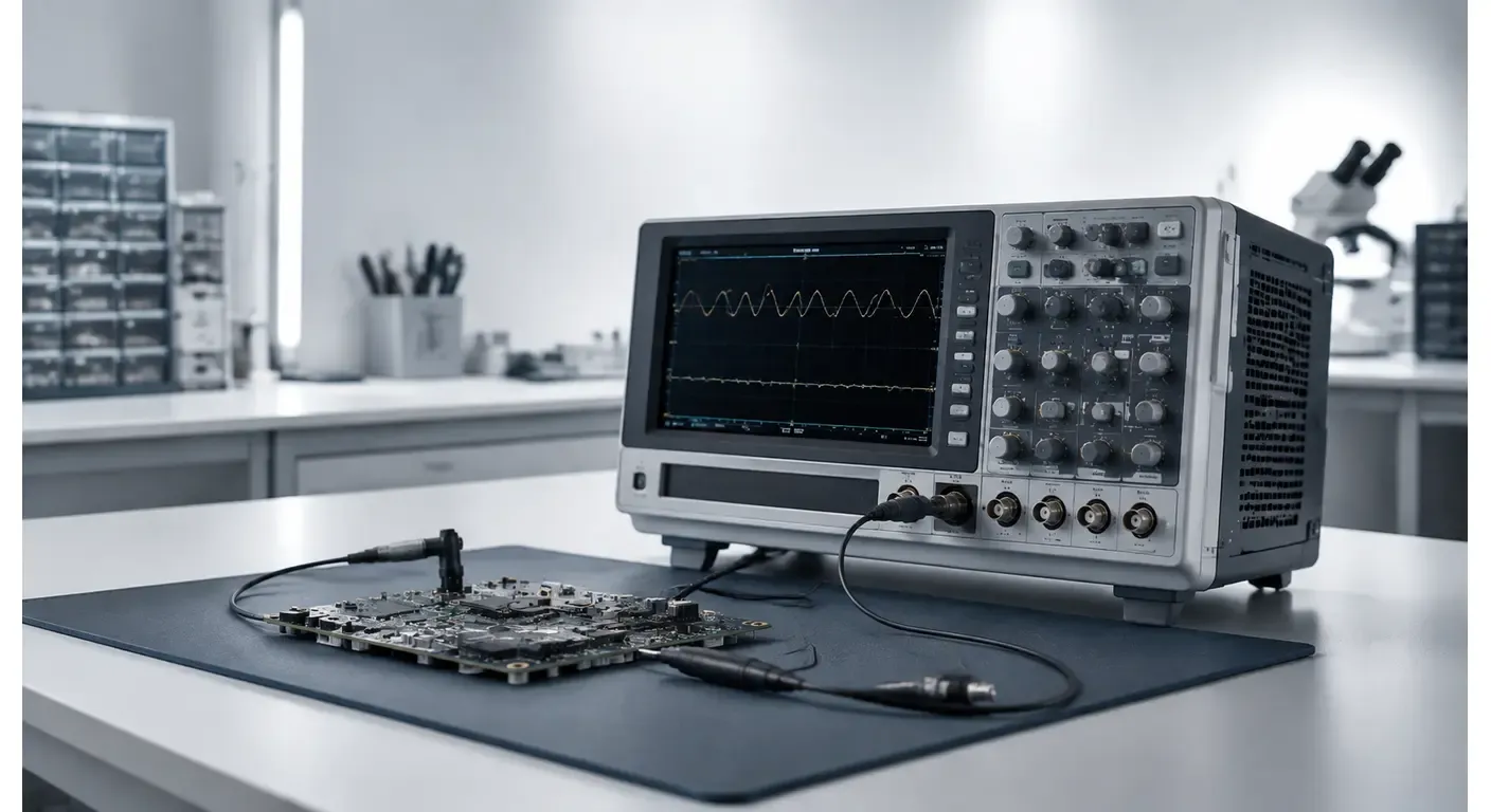
An oscilloscope displays voltage as a function of time, making circuit behavior visible in a way no other instrument matches. Analog and digital oscilloscopes pursue that same objective, but they reach it through fundamentally different architectures: an analog instrument deflects an electron beam in real time, while a digital instrument samples the signal, converts it into numbers and reconstructs the waveform from memory.
That single architectural difference determines everything else. Storage, automatic measurement, pre-trigger viewing, spectral analysis and data export all depend on the signal existing as data. Aliasing, dead time and configuration complexity are the costs that come with it.
Digital oscilloscopes are the industry standard today. Analog oscilloscopes retain value in a narrow set of situations, and knowing exactly where those situations lie is more useful than treating the technology as obsolete. This comparison sits within our complete Test & Measurement guide, which covers the rest of the instruments on a bench.
Analog vs Digital Oscilloscope: Quick Comparison
The table below summarizes the differences that most often determine the choice between the two technologies.
| Criterion | Analog Oscilloscope | Digital Oscilloscope |
|---|---|---|
| Signal processing | Direct amplification and beam deflection, no conversion | Sampling, ADC conversion and digital processing |
| Display technology | Cathode ray tube with phosphor persistence | Color LCD with digitally rendered trace |
| Waveform storage | None on standard models; the trace fades as it is drawn | Native; acquisitions are held in memory and can be saved |
| Measurement capabilities | Manual reading against the graticule | Automatic amplitude, timing and statistical measurements |
| Ease of use | Few controls, each with a direct effect on the display | Broader capability, menu-driven, longer learning curve |
| Best applications | Repetitive analog signals, basic servicing, teaching | Embedded systems, power electronics, automotive, industrial, research |
The rest of this article explains why these differences exist and what they mean in practice.
What Does an Oscilloscope Do?
An oscilloscope plots voltage on the vertical axis against time on the horizontal axis. From that graph an engineer derives amplitude, DC offset, period and frequency, rise and fall time, pulse width, duty cycle, overshoot, ringing and phase relationships between channels. Non-electrical quantities become measurable through the appropriate transducer or probe.
The value lies in showing behavior rather than a result. A multimeter reports that a supply rail measures 3.28 V; an oscilloscope reveals the 40 mV of switching ripple riding on it, or the brief collapse to 2.9 V each time a motor starts. That distinction is examined in our comparison of a digital multimeter and an oscilloscope.
Both analog and digital instruments perform this core function. Where they diverge is in what happens to the signal between the probe tip and the screen — and in what the instrument can do with the signal once it is displayed. Readers new to this class of instrument will find the fundamentals covered in our reference article on what an oscilloscope is and how it works.
How Analog and Digital Oscilloscopes Work
How an Analog Oscilloscope Works
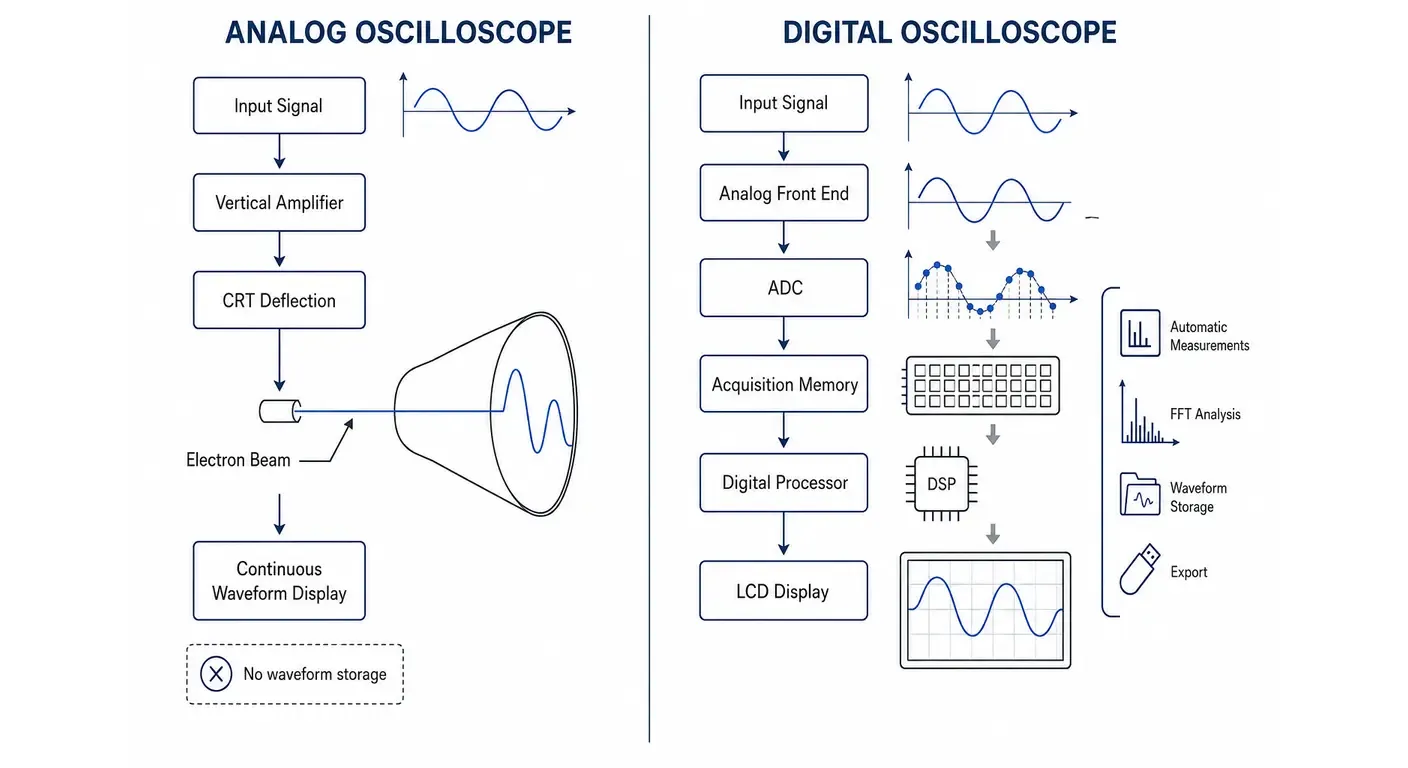
An analog oscilloscope is a direct-display instrument. The input signal is amplified or attenuated and applied to the vertical deflection plates of a cathode ray tube. A timebase circuit sweeps the electron beam horizontally at a controlled rate, and the trace appears wherever the beam strikes the phosphor.
There is no intermediate representation. What appears on screen is the amplified signal itself, deflecting the beam in real time. Provided the signal repeats and the trigger circuit starts each sweep at the same point, successive sweeps overlap and the waveform appears stationary.
The consequence for measurement is straightforward: the instrument can display a signal, but it cannot retain one. Once the beam has passed, the trace fades, and any parameter of interest must be read from the graticule while the signal is still present.
How a Digital Oscilloscope Works
A digital oscilloscope replaces the deflection path with a signal chain built around an analog-to-digital converter. The conditioned signal is sampled at regular intervals, each sample is converted into a numerical value, and those values are written into acquisition memory. A processor then interpolates between sample points, performs any requested measurements, and renders the result on an LCD.
What appears on screen is a reconstruction of the signal built from stored data. Three specifications govern how faithful that reconstruction is: oscilloscope bandwidth, which sets how much of a fast edge survives the analog front end; sample rate, which determines how finely the signal is captured in time; and vertical resolution, the number of ADC bits available to divide the amplitude range.
Why the Architecture Difference Matters
Nearly every practical difference between the two technologies follows from the presence or absence of acquisition memory.
Because a digital instrument writes samples into memory continuously and in a circular fashion, it already holds data from before the trigger event occurred. Pre-trigger viewing is a direct consequence of the architecture, and it has no analog equivalent. For the same reason, a single-shot event can be frozen and examined afterward, automatic measurements can be computed over many acquisitions, and the captured waveform can be transformed by FFT, filtered, decoded or exported.
An analog instrument gains something in exchange. It draws every sweep it triggers on, with no processing interval during which it is blind to the input, and the phosphor glows more brightly where the beam passes more often — an intensity gradient that conveys how frequently each part of the signal occurs. It also cannot alias, because nothing is sampled.
Analog vs Digital Oscilloscope: Full Technical Comparison
| Characteristic | Analog Oscilloscope | Digital Oscilloscope |
|---|---|---|
| Signal acquisition | Continuous; the signal is displayed as it arrives | Discrete; the signal is sampled at fixed intervals |
| Signal processing | Analog amplification only, no conversion stage | ADC conversion followed by digital signal processing |
| Display | Cathode ray tube; brightness varies with beam dwell time | Color LCD; trace rendered from memory contents |
| Bandwidth | Commonly tens to a few hundred MHz on classic bench models | From tens of MHz on entry models to tens of GHz on high-end instruments |
| Sampling rate | Not applicable; no sampling occurs | A primary specification; determines time resolution and aliasing risk |
| Memory depth | Not applicable; no acquisition memory | Determines how long a capture can run at a given sample rate |
| Triggering | Edge, delayed sweep and video triggering; no pre-trigger view | Edge, pulse width, runt, slew rate, serial protocol and zone triggers, with pre-trigger data |
| Storage | None on standard models; requires a storage CRT or a camera | Waveforms held in memory, saved to file and recalled |
| Automated measurements | None; parameters are read manually from the graticule | Amplitude, timing, statistical and mask measurements computed continuously |
| Data analysis | Visual inspection only | FFT, waveform math, digital filtering, protocol decode, mask testing |
| Portability | Bulky; the CRT and its high-voltage supply define size and weight | Bench, portable and handheld formats, often battery powered |
| Applications | Repetitive analog signals, teaching, basic audio and RF servicing | Embedded development, power electronics, automotive, industrial, research |
Three rows deserve a note. Memory depth has no analog counterpart at all: it sets how long a digital instrument can record before it must either stop or reduce its sample rate, and it is what makes long, slow, non-repeating events capturable. Triggering is where the two technologies diverge most sharply in practical use, because isolating a specific fault condition — a runt pulse, a particular bus address — is what turns an intermittent problem into a reproducible one. Sampling rate is the specification that introduces a failure mode absent from analog instruments, discussed below.
Advantages and Limitations of Analog Oscilloscopes
Advantages
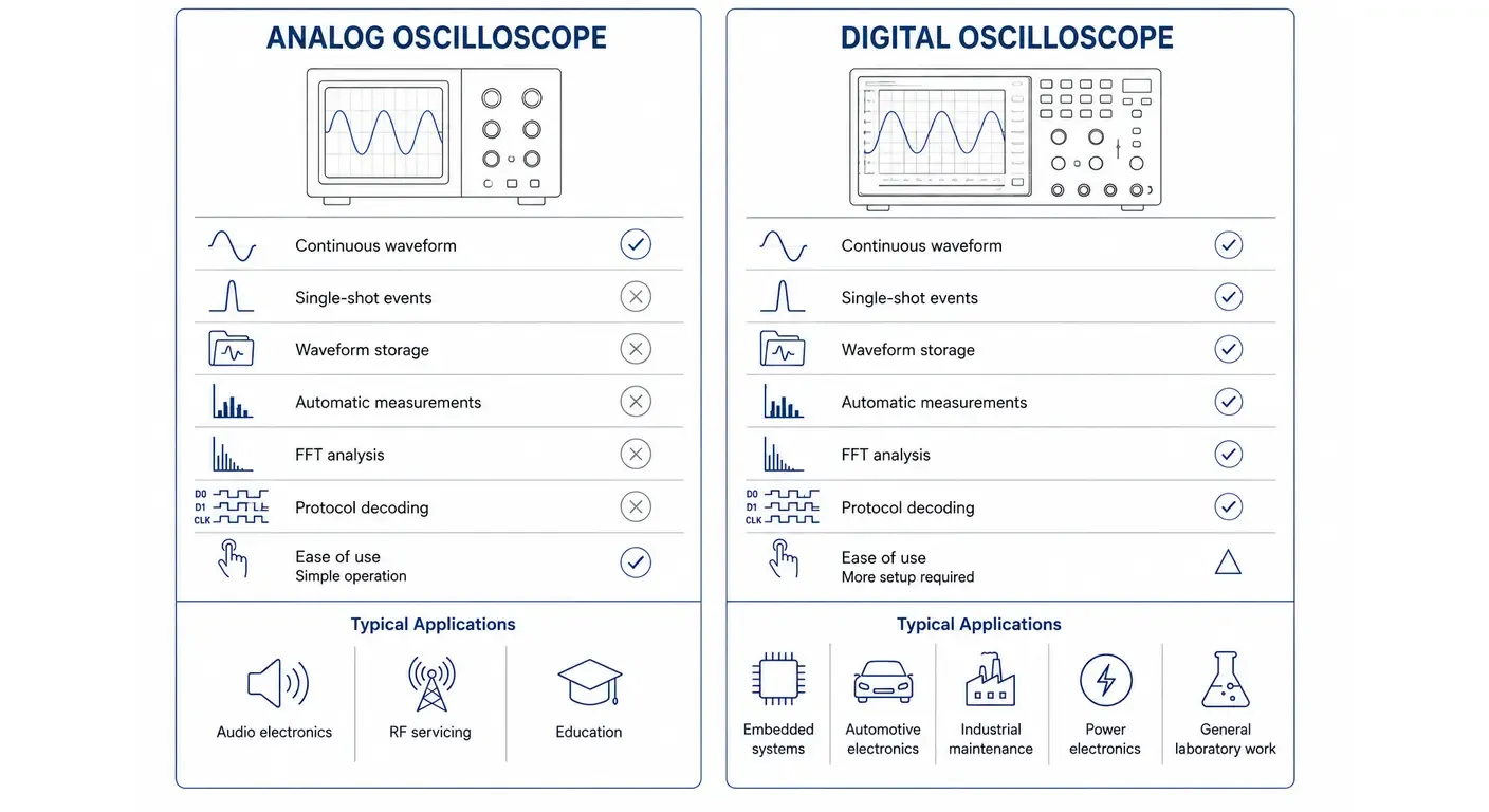
Continuous display with no dead time. Every triggered sweep is drawn. A rare glitch occurring once every few thousand cycles will eventually appear, and the phosphor renders it as a faint trace against the bright main waveform. Digital instruments must process each acquisition before arming again, leaving short intervals during which the input is not observed.
Immediate response. The trace follows the signal with no acquisition or rendering delay, which suits alignment work where a control is adjusted while the display is watched.
Simple, transparent operation. Vertical sensitivity, timebase and trigger level are the essential controls, each with an unambiguous physical effect. No automatic setting can silently alter what is displayed.
No aliasing. Without sampling, the instrument cannot display a frequency that is not present in the signal. Beyond its bandwidth the trace simply attenuates.
Limitations
No waveform storage. A power-up transient, an intermittent fault or a single serial frame cannot be retained. If it is not caught by eye as it happens, it is gone — the single most consequential limitation compared with a digital instrument.
Manual measurement. Amplitude and timing are read by counting graticule divisions and multiplying by the range settings. Measurement uncertainty depends on the operator as much as on the instrument.
Bulky hardware. The CRT, its high-voltage supply and the associated shielding make portable operation impractical.
No modern analysis or documentation. There is no FFT, no protocol decode, no screenshot capture and no data export. Recording a measurement means photographing the screen.
Advantages and Limitations of Digital Oscilloscopes
Advantages
Waveform capture and storage. Any acquisition can be frozen, zoomed into and saved. Single-shot capture turns intermittent faults from a matter of luck into a matter of configuring the right trigger and waiting.
Automatic measurements. Rise time, frequency, duty cycle, RMS amplitude and dozens of other parameters are computed continuously, usually with statistics across many acquisitions that reveal variation the eye would not detect.
Advanced triggering. Beyond edge triggering, digital instruments isolate specific conditions: pulses narrower than a defined width, runt pulses that fail to reach a logic threshold, or a particular address on an I²C or CAN bus.
Analysis functions. FFT converts the trace into a frequency spectrum, exposing noise sources and harmonic content. Waveform math, digital filtering and mask testing extend the instrument well beyond display.
Connectivity and documentation. Screenshots, CSV export and remote control make results reproducible and suitable for formal test reports — something an analog instrument cannot support in any form.
Limitations
Aliasing. If the sample rate is too low relative to the signal frequency, the reconstructed waveform can appear as a slower signal not present in the circuit. The display looks entirely plausible, which is what makes the error dangerous.
Greater operational complexity. Acquisition modes, interpolation settings and memory management all influence what appears on screen, and an incorrectly configured acquisition mode can smooth away the detail being investigated. Our guide on how to use an oscilloscope covers the settings that matter most.
Dead time between acquisitions. Modern architectures reduce this substantially, with high update rates reaching hundreds of thousands of waveforms per second, but a strictly continuous view of the input is not achievable.
Cost of advanced capability. Entry-level instruments are inexpensive, but deep memory, high sample rates, higher vertical resolution and protocol decode raise the price considerably.
Which Oscilloscope Is Best for Different Applications?
Electronics Education
Digital is the standard teaching instrument, because students will encounter digital equipment throughout their careers and benefit from learning measurement functions early. Analog retains one pedagogical strength: the relationship between trigger, timebase and displayed trace is physically obvious rather than mediated by software, which makes triggering easier to grasp the first time. Where both are available, an analog instrument teaches the concept and a digital instrument teaches the practice.
Circuit Debugging
The determining question is whether the fault repeats. For a repetitive analog signal — an audio stage, a linear supply, an oscillator — an analog oscilloscope is entirely adequate and displays the waveform without configuration. For anything intermittent, digital is the only practical choice, because diagnosis depends on capturing an event that may not recur while the engineer is watching.
Embedded Systems
Digital, without qualification. Firmware debugging requires single-shot capture, deep memory, pre-trigger data and serial protocol decode for buses such as UART, I²C, SPI and CAN. None of these exist on an analog instrument. Where many logic signals must be observed simultaneously, the trade-off between instrument classes is explained in our comparison of a logic analyzer and an oscilloscope.
Industrial Maintenance
Digital, in portable or handheld form. Battery operation, rugged enclosures and isolated inputs allow safe measurement on drives and control panels where channel grounds sit at different potentials. Stored waveforms also serve as a maintenance record: a sensor output measured today can be compared against a reference captured when the machine was commissioned. An analog instrument offers neither the portability nor the record.
Automotive Electronics
Digital. Automotive signals are frequently slow but non-repeating — a cranking voltage profile, an injector pulse train, a single CAN frame. Capturing them requires long acquisition times at adequate sample rates, which is a memory depth problem that analog instruments cannot address at all.
Laboratory Research
Digital, with high bandwidth, deep memory and higher vertical resolution. Jitter analysis, eye diagrams, spectral measurements and statistical characterization all require the acquired data to exist as numbers. Analog instruments remain in some laboratories as secondary bench equipment, but not as the primary measurement platform.
How to Choose Between an Analog and a Digital Oscilloscope
Four questions resolve most selection decisions.
| Question | If the answer is… | Appropriate instrument |
|---|---|---|
| Does the signal repeat continuously? | No — the event occurs once or intermittently | Digital, for single-shot capture |
| Must the captured waveform be retained? | Yes — for later analysis or comparison | Digital, for acquisition memory |
| Does the circuit contain digital buses or logic? | Yes — UART, I²C, SPI, CAN or similar | Digital, for advanced triggering and decode |
| Must the result be documented or shared? | Yes — test reports, records, collaboration | Digital, for export and screenshots |
If all four answers are no — a repetitive analog signal, observed live, on a circuit without digital buses, with no documentation requirement — either technology will do the work, and an analog instrument may be preferable for its immediacy and simplicity. A single yes points to a digital instrument.
Are Analog Oscilloscopes Still Relevant?
Analog oscilloscopes became uncommon for reasons that had little to do with waveform quality. Digital instruments delivered storage, automatic measurement, documentation and connectivity in a smaller and lighter package, and the cost of digital acquisition hardware fell steadily. Major test and measurement manufacturers no longer list analog oscilloscopes in their current catalogs, and the technology now circulates almost entirely through the secondhand market.
They remain useful in a narrow set of situations. A well-maintained analog scope is an inexpensive and capable instrument for repetitive analog signals, particularly in audio and RF servicing. Its continuous, dead-time-free display retains a certain diagnostic character when hunting for infrequent disturbances on a repetitive waveform. For teaching the fundamentals of triggering and timebase, the directness of the instrument is a genuine advantage. And where one has been in service for decades, replacing a working instrument is rarely a priority.
The practical arguments against acquiring one are equally clear. Aging CRTs lose brightness, high-voltage supplies and electrolytic capacitors fail, spare parts are scarce, and calibration services for discontinued models are increasingly difficult to obtain. There is no path to protocol decode, spectral analysis or exportable measurement records.
It is also worth noting that modern digital oscilloscopes with high waveform update rates and intensity-graded displays have recovered much of what made analog instruments useful for spotting rare events. The residual advantage of an analog scope in that specific task is narrower today than its reputation suggests.
Conclusion
Analog and digital oscilloscopes pursue the same objective through fundamentally different architectures, and that architecture determines their capabilities.
Analog oscilloscopes remain useful for repetitive analog signals, basic servicing work and teaching environments where the directness of the display has instructional value. They show the signal continuously, with no sampling and therefore no aliasing, but they cannot store what they show.
Digital oscilloscopes provide storage, automatic measurement, advanced triggering, spectral and protocol analysis, and exportable results. For any work involving digital systems, transient events or documented test results, these are not conveniences but prerequisites. The cost is a more complex instrument and a set of sampling-related failure modes the operator must understand.
Selecting an oscilloscope is therefore a question of matching the instrument to the measurement objective, not of establishing which technology is superior. Define what must be measured, how fast it changes, whether it repeats, and whether the result must be recorded — those four answers point clearly to the right instrument.
An oscilloscope is only as accurate as the complete measurement system it forms together with the probe and the technique used to apply it, and this holds equally for analog and digital instruments.
Is a digital oscilloscope better than an analog oscilloscope?
For the large majority of modern engineering work, yes. A digital oscilloscope stores waveforms, captures single-shot events, performs automatic measurements and exports results, none of which a standard analog instrument can do. An analog oscilloscope retains a narrow advantage in continuous, dead-time-free display of repetitive signals.
Do engineers still use analog oscilloscopes?
Some do, mainly in audio and RF servicing, in teaching laboratories, and where a working instrument has been in service for many years. They are no longer purchased for new laboratory equipment, and major manufacturers no longer offer them.
Why are digital oscilloscopes more popular?
They store acquisitions in memory, which enables everything that follows: single-shot capture, pre-trigger viewing, automatic measurements, FFT analysis, serial protocol decode, screenshots and data export. They are also smaller, lighter and available across a wide price range.
What are the disadvantages of digital oscilloscopes?
Aliasing is the most significant, since an undersampled signal can be displayed as a slower waveform that does not exist in the circuit. Digital instruments also have dead time between acquisitions, present a more complex menu-driven interface, and become expensive once deep memory and analysis options are required.
Which oscilloscope is best for beginners?
An entry-level digital oscilloscope. It teaches the measurement functions used throughout modern engineering practice, and the ability to freeze and examine a waveform makes learning considerably easier. Bandwidth of 100 MHz with two or four channels covers most learning work comfortably.
Can a digital oscilloscope replace an analog oscilloscope?
In nearly all cases, yes. A digital instrument reproduces the core function of displaying voltage against time and adds storage and analysis. The one characteristic it does not fully replicate is the strictly continuous display of an analog scope, although high waveform update rates have narrowed that gap substantially.
Related articles
Electronics18 min read
Function Generator vs Arbitrary Waveform Generator: What You Are Buying
Three names, two architectures: how DDS and point-by-point playback differ, what the labels hide, and how to read the architecture off a datasheet.
Electronics23 min read
How to Choose a Signal Generator: Getting the Signal You Asked For
How to turn a required stimulus into datasheet requirements: the load the instrument assumes, bandwidth against sample rate, reconstruction and vertical resolution.
Electronics22 min read
How to Choose a Multimeter: A Specification-Led Buying Guide
Choose a multimeter by the errors it introduces: burden voltage, input loading, AC bandwidth, safety category and accuracy on the reading you actually take.
Electronics16 min read
How to Use a Thermal Camera: Getting Readings You Can Trust
A thermal camera always shows a number. Learn the checks — emissivity, reflected temperature, focus and spot size — that decide whether it is a measurement.