Oscilloscope vs Logic Analyzer: Key Differences and How to Choose
Oscilloscope vs logic analyzer: how each instrument measures signals, where each one fails, and how to choose the right tool for analog, digital and mixed-signal debugging.
By YDT EditorialUpdated 29 min read
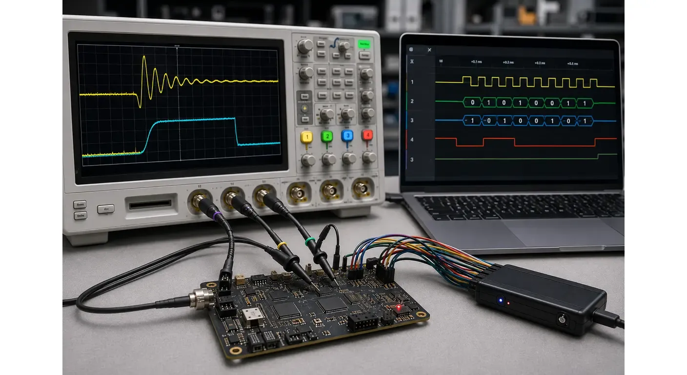
Two engineers look at the same misbehaving board. One clips an oscilloscope probe onto a single line and studies the shape of the signal. The other drops a sixteen-channel logic analyzer across the whole bus and studies the order of events. An hour later, one of them has found the fault and the other has confirmed that everything looks fine.
Which one wasted the hour depends entirely on what was actually broken.
That is the real subject of this article. An oscilloscope answers what does this signal actually look like? A logic analyzer answers what did this bus actually do? Choosing between them has very little to do with price or channel count, and everything to do with matching the instrument to the failure mechanism you are chasing. Both instruments are part of our complete Test & Measurement guide, which covers the rest of the bench.
Oscilloscope vs Logic Analyzer: Quick Overview
Key differences at a glance
Before the theory, the short version — the table most engineers actually need at the moment they are deciding which instrument to unplug from the shelf.
| If you need to… | Reach for… |
|---|---|
| Check whether a rail is clean or a signal is distorted | Oscilloscope |
| Find ringing, overshoot or a slow edge | Oscilloscope |
| Measure rise time, propagation delay or timing margin | Oscilloscope |
| Decode SPI or I²C traffic over thousands of transactions | Logic Analyzer |
| Watch 16 GPIO lines change state simultaneously | Logic Analyzer |
| Trigger on a specific pattern across a parallel bus | Logic Analyzer |
| Find out why a valid-looking digital signal is failing | Mixed Signal Oscilloscope |
Now the reason behind it.
An oscilloscope samples voltage with an analog-to-digital converter (ADC) of typically 8 to 12 bits, producing a waveform that represents the real electrical shape of the signal. Amplitude, rise time, noise, overshoot and distortion are all preserved, within the limits of the instrument’s bandwidth and sample rate.
A logic analyzer samples the same wire with a single comparator. The comparator decides against a threshold: a user-configured voltage that separates logic low from logic high. The result is one bit per channel per sample. Everything about the analog shape is thrown away at the input, and what remains is a precise record of when each line changed state — across many channels at once, for a long time.
That one architectural decision — many bits on few channels versus one bit on many channels — explains almost every other difference between the two instruments. Keep it in mind and the rest of this article is mostly consequences.
Which instrument solves which problems?
| Characteristic | Oscilloscope | Logic Analyzer |
|---|---|---|
| Measured quantity | Voltage as a continuous analog value | Logic state relative to a configured threshold |
| Vertical resolution | Nominally 8-bit (256 levels), 10 to 12-bit on high-resolution models | 1 bit per channel |
| Typical channel count | 2 or 4 analog channels | 8, 16, 32 or more, up to 100+ on high-end systems |
| Typical sample rate | Hundreds of MSa/s to several GSa/s | Tens of MSa/s to several GSa/s, depending on class |
| Bandwidth concept | Analog front-end bandwidth defines the fastest edge visible | Threshold comparator response and sample rate define timing resolution |
| Memory efficiency | High: many bits per sample, per channel | Very high: 1 bit per sample, per channel, enabling long captures |
| Triggering | Edge, pulse width, runt, glitch, serial pattern | Multi-channel state and pattern conditions, bus sequences |
| Protocol decoding | Available on most modern models, usually on 1 to 4 buses | Core capability, often across many buses simultaneously |
| Primary strength | Signal quality and analog behavior | System behavior and multi-signal timing |
| Primary blind spot | Cannot observe many digital lines at once | Cannot observe anything about signal shape |
What Does an Oscilloscope Measure?
Analog voltage over time
Picture a board that runs perfectly on the bench and resets itself every few minutes in the field. The firmware is identical. The schematic has not changed. Nothing in the code explains it.
This is the class of problem an oscilloscope exists for, because the fault is not in what the system did — it is in what the electricity did.
An oscilloscope displays voltage on the vertical axis and time on the horizontal axis. The input signal passes through an attenuator and amplifier, then into an ADC that samples it at regular intervals, and the stored samples are reconstructed into the waveform on screen.
Because the ADC resolves amplitude into hundreds or thousands of levels, it preserves information that has no digital equivalent: how fast an edge rises, how far it overshoots, how long it rings before settling, how much noise rides on a supply rail, and whether a logic high actually reaches a valid V_IH level at the receiver. In the resetting-board example, that is where the answer usually lives — a brownout on a rail during a load transient, invisible to any instrument that only records ones and zeros.
This is the information that determines whether a digital circuit works reliably, or merely works today.
Bandwidth, sampling rate, and waveform visualization
Bandwidth is the frequency at which the oscilloscope’s front end attenuates a sine wave by 3 dB. It is a property of the analog signal path, and it sets a hard limit on the fastest transition the instrument can represent faithfully. The familiar approximation:
BW ≈ 0.35 / t_rise
That 0.35 assumes a Gaussian frequency response, which is characteristic of most instruments below roughly 1 GHz. Higher-bandwidth oscilloscopes generally use a maximally flat response, where the appropriate constant is closer to 0.40–0.45. Manufacturer documentation states which applies — and it is worth checking rather than assuming.
The practical consequence is easier to see through the error it produces. The instrument and the signal contribute rise time in quadrature:
t_measured ≈ √(t_signal² + t_scope²)
So suppose you put a 100 MHz oscilloscope — intrinsic rise time about 3.5 ns — on a signal whose true edge is also 3.5 ns. The screen reports roughly 4.9 ns. You are 41% wrong, and nothing on the display suggests it. Swap in a 350 MHz instrument, intrinsic rise time near 1 ns, and the same measurement returns about 3.6 ns: an error near 4%.
That is where the conventional guideline comes from — pick an instrument three to five times faster than the edge under test, or with three to five times the highest frequency component of the signal.
Sample rate is a separate specification, expressed in samples per second, and it governs how finely the waveform is captured in time. Manufacturers generally recommend a sample rate several times higher than the instrument bandwidth so the reconstruction algorithm has enough points to work with. Bandwidth and sample rate must both be adequate; neither rescues the other.
Memory depth determines how many samples the instrument can store. In the abstract that sounds like a minor specification. In practice, imagine you are hunting a fault that appears once every five seconds — suddenly memory depth matters far more than bandwidth, because capture duration equals memory depth divided by sample rate. A shallow memory forces the oscilloscope to drop its sample rate as you increase the timebase, which is exactly why an instrument that looks fast on a datasheet can fall apart the moment you zoom out to see a whole transaction.
Typical engineering applications
Oscilloscopes are the right instrument whenever the physics of the signal is under investigation: switching-converter behavior, power-rail noise and transient response, sensor and amplifier outputs, motor drive waveforms, crystal and PLL startup, EMI investigation, probe-level signal integrity work, and any situation where a digital signal is suspected of being electrically marginal rather than logically wrong.
What Does a Logic Analyzer Measure?
Digital logic states
Now a different kind of morning. A new board comes back from assembly, firmware is flashed, and the SPI sensor returns nothing at all. The scope shows activity on the clock line — so the peripheral is running — but four channels are not enough to see the chip select, the clock, the outgoing command and the returning data at the same time, and you have already run out of inputs.
This is where the logic analyzer earns its place on the bench.
It compares each input against its configured threshold voltage and records a single bit. Because the threshold is adjustable, the same instrument serves 5 V, 3.3 V, 1.8 V or lower logic families.
Two acquisition modes exist. In timing mode (asynchronous), the instrument samples with its own internal clock, independent of the circuit — the mode used for general debugging, with timing resolution equal to one sample period. In state mode (synchronous), it samples on an edge of a clock supplied by the circuit under test, capturing exactly the data the receiving device latches. State mode is invaluable on memory buses and clocked parallel interfaces, where the question is what value was latched, not when did the line move.
Multi-channel timing analysis
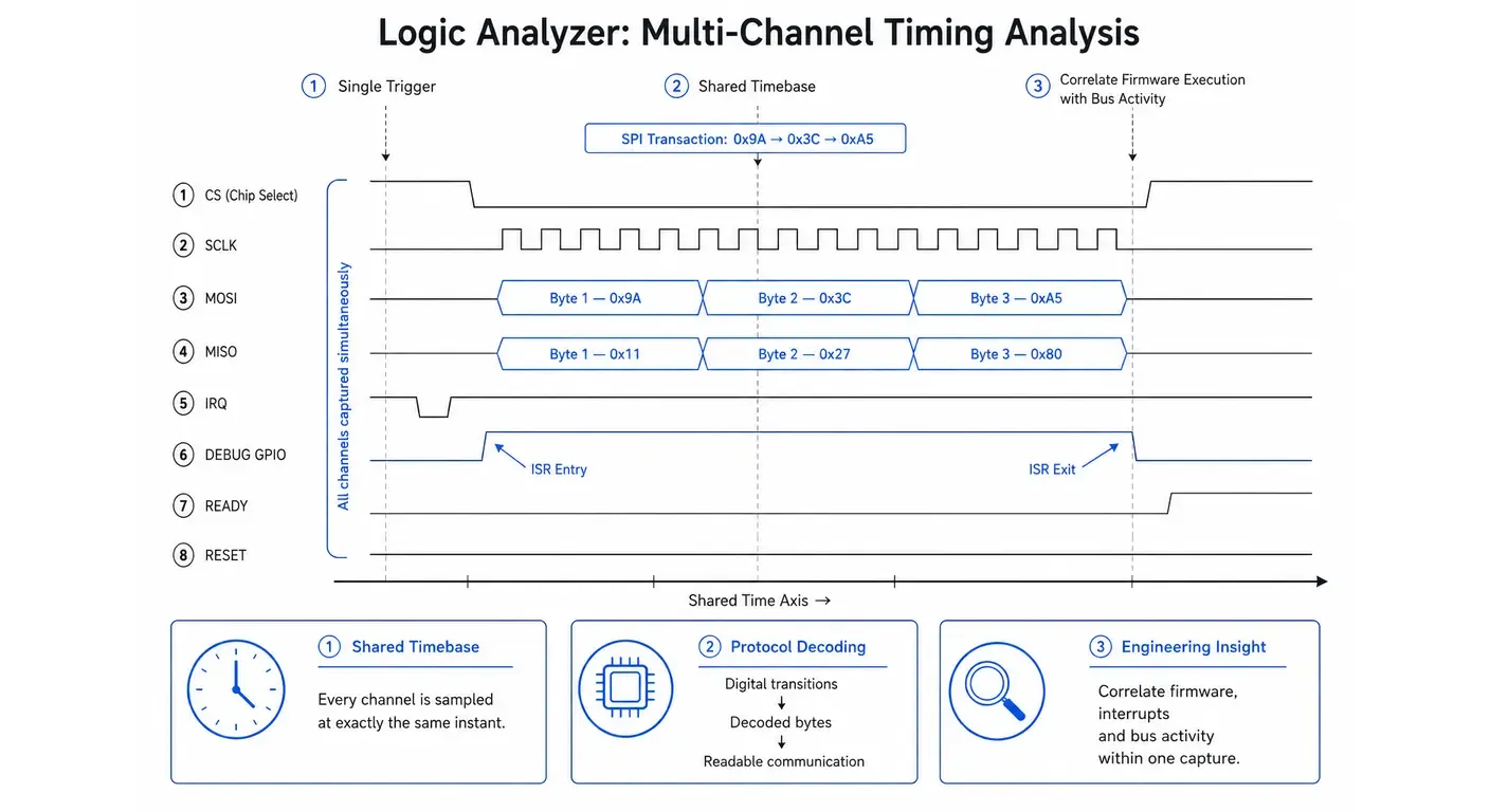
The defining advantage is simultaneity. Sixteen, thirty-two or more channels are captured against a single timebase, so the relationship between a chip select, a clock, several data lines, an interrupt request and a firmware-controlled debug GPIO can all be examined in one capture. That last one is worth emphasizing: toggling a spare pin at the top and bottom of an interrupt handler, then watching it alongside the bus, turns the analyzer into a view of your firmware’s execution timing as well as its output.
Because each channel consumes one bit per sample, memory is used far more efficiently than in an oscilloscope. A logic analyzer can record millions of bus events across seconds of real time — long enough to catch the intermittent fault that shows up once every few thousand transactions.
Protocol decoding capabilities
Most logic analyzers include protocol decoders that convert captured logic states into readable transactions: SPI words with their chip-select framing, I²C addresses with ACK and NACK bits, UART bytes with parity and framing errors, CAN frames with identifiers and CRC fields. Many decode several buses in parallel within the same capture, which is precisely what you need when the bug lives in the interaction between two peripherals rather than in either one alone.
One caution: decoding is only as good as the capture beneath it. A decoder applied to an undersampled or badly thresholded acquisition produces confident, incorrect output — and confident incorrect output is considerably more expensive than no output at all.
Typical engineering applications
Firmware bring-up, bus protocol verification, state machine and FPGA debugging, memory interface analysis, boot sequence investigation, and any fault whose signature is a wrong sequence rather than a wrong shape.
Oscilloscope vs Logic Analyzer: Technical Comparison
Analog versus digital measurements
An oscilloscope measures a physical quantity. A logic analyzer measures an interpretation of a physical quantity. That interpretation happens in a comparator whose decision is binary and irreversible: once the sample is stored, how close the signal came to the threshold is gone forever. No amount of post-processing brings it back.
Number of input channels
Oscilloscopes are usually limited to two or four analog channels, because each one needs a complete analog front end and, in most architectures, its own ADC. Logic analyzer channels are a comparator and a slice of memory, which is why 16 or 32 channels are unremarkable and high-end systems reach well beyond a hundred.
Sampling rate and bandwidth
Oscilloscope sample rates in the GSa/s range are common even mid-range. Logic analyzers vary enormously: inexpensive USB units may sample at tens of MSa/s, professional instruments reach GSa/s in timing mode. The working guideline is to sample at least four to ten times faster than the fastest edge rate of interest, since the uncertainty on any recorded transition is one full sample period.
Run the numbers once and the rule stops being abstract. A 24 MSa/s USB analyzer carries roughly 42 ns of timing uncertainty. On a 100 kHz I²C bus, where a bit lasts 10 µs, that is invisible. On a 25 MHz SPI link, where the entire clock period is 40 ns, you are trying to verify setup and hold margins with an instrument whose uncertainty exceeds the thing you are measuring.
Vertical resolution
An 8-bit oscilloscope resolves its vertical range into 256 levels; 12-bit models resolve it into 4096. Those figures are nominal, and the distinction matters. Once front-end noise, ADC nonlinearity and distortion are accounted for, the effective number of bits (ENOB) of a typical 8-bit oscilloscope falls to roughly 6 to 7 across its full bandwidth. Usable amplitude resolution is therefore coarser than the datasheet number implies — which you discover the first time you try to measure 20 mV of ripple sitting on a 12 V rail.
A logic analyzer resolves the vertical axis into two states. That is not a deficiency, it is the design intent — but it defines the outer boundary of what the instrument can ever tell you.
Triggering capabilities
A trigger is the condition that tells the instrument when to capture. Oscilloscope triggers act mainly on the shape and timing of one or two signals: rising edge, pulse width, runt pulse, glitch, or a serial pattern on a decoded bus. Logic analyzer triggers act on the state of many channels at once, and frequently on sequences — trigger when this address appears on the bus and the write strobe is asserted and the acknowledge never returns.
For intermittent system-level faults, trigger capability decides the outcome far more often than sample rate does. An instrument that captures the wrong ten milliseconds at a gigasample per second has told you nothing.
Memory depth
Capture duration is memory depth divided by sample rate. Because logic analyzers store one bit per channel per sample, they achieve very long capture windows without extravagant memory. Oscilloscopes must store full-resolution samples, and on many models the available memory is shared between active channels — enabling a fourth channel can quietly halve the record length on the other three, usually without announcing it.
Two logic analyzer features push the advantage further. Transitional storage (also called run-length or timing-zoom storage) records a sample only when a channel changes state, which is extremely efficient on buses that sit idle most of the time. Glitch capture latches any pulse narrower than one sample period, so a short anomaly is flagged even though its width and shape are not measured. Glitch capture partly offsets the instrument’s blindness to brief events — but it tells you only that something happened, never what it looked like.
Timing accuracy
Within its bandwidth, an oscilloscope places an edge with sub-sample precision, because interpolation uses the amplitude information surrounding the transition. A logic analyzer in timing mode cannot: it knows only which sample first reported the new state.
Sub-sample precision is not unlimited accuracy, though, and this catches people out. Absolute and delta-time measurements are also bounded by timebase accuracy — typically specified in parts per million, with ±25 ppm representative of bench instruments — and by trigger jitter, often a few picoseconds RMS. Measure across a 1 ms interval and ±25 ppm alone contributes ±25 ns of uncertainty before anything else is considered. For propagation delay, skew and setup/hold verification the oscilloscope is still the more accurate instrument, provided it has the bandwidth. Just check the timebase specification, not only the sample rate.
Protocol analysis
Both instrument families decode serial protocols; the difference is scale and context. An oscilloscope decodes a small number of buses while simultaneously showing their electrical quality — what you want when a bus fails because of loading or reflections. A logic analyzer decodes many buses over long periods — what you want when a bus fails because of firmware sequencing.
Measurement limitations
A logic analyzer cannot show ringing, overshoot, undershoot, slow or non-monotonic edges, ground bounce, insufficient drive strength, or a signal parked just above the threshold. Every one of those produces intermittent digital faults. So if a bus works at low speed and fails at high speed, or works on one board and not the next one off the line, expect the logic analyzer to report that everything looks completely normal. It is not malfunctioning. It is telling you the truth about the only thing it can see.
The reverse limitation is just as real. A four-channel oscilloscope cannot tell you what a sixteen-bit parallel bus did during a boot sequence, and its memory will not hold several seconds of traffic at full sample rate.
And there is a limitation common to both that costs more debugging hours than either of the above: connecting the instrument changes the circuit. A 10:1 passive probe typically presents 10 to 15 pF of input capacitance, and a logic analyzer pod applies comparable capacitance to every connected channel at once — frequently through long unshielded flying leads that contribute inductance as well. On a bus already close to its rise-time limit, or on a high-impedance node, that is enough to slow edges and alter behavior. If a fault vanishes when you unplug the analyzer, or only appears once you connect it, treat it as a loading problem until proven otherwise. The instrument has become part of the circuit.
Common Engineering Use Cases
Debugging power electronics
Switching converters, gate drive circuits, inrush behavior and rail sequencing are analog problems from beginning to end. Dead time, gate ringing, diode reverse recovery and switching losses all live in the waveform shape. Oscilloscope territory exclusively — a logic analyzer contributes nothing here.
Troubleshooting embedded systems
Embedded faults divide cleanly along one line. If the microcontroller is executing the wrong sequence, missing an interrupt or configuring a peripheral incorrectly, the logic analyzer finds it quickly. If the microcontroller is executing perfectly and the signal simply never arrives intact at the far end of the board, only the oscilloscope will show why — and signal integrity failures of that kind account for a large share of the bugs that survive code review intact.
Verifying SPI, I²C, UART and CAN communications
For functional verification — correct addressing, correct framing, correct acknowledgment, correct spacing between transactions — a logic analyzer with protocol decoding is the efficient choice, especially when several devices share a bus.
For electrical verification, you need the oscilloscope. I²C is the classic demonstration. The bus uses open-drain drivers and passive pull-up resistors, so the rising edge is an RC exponential set by the pull-up value and total bus capacitance. The specification caps that rise time at 1000 ns in Standard mode (100 kHz) and 300 ns in Fast mode (400 kHz). A pull-up chosen for low power, on a bus carrying several devices and a few hundred picofarads, can comfortably satisfy the first limit and violate the second. Result: the bus works at 100 kHz, fails at 400 kHz, and the logic analyzer reports valid transactions in both cases because both cross the threshold eventually.
CAN deserves its own paragraph, because the usual advice quietly does not apply. Suppose a network runs flawlessly at 125 kb/s and starts throwing errors at 1 Mb/s — a genuinely common scenario in vehicle and industrial systems. Your first instinct is to put a logic analyzer on the bus. You cannot: the CAN physical layer is a differential pair (CAN_H and CAN_L), and a single-ended analyzer has nothing meaningful to compare against. Standard practice is to probe the transceiver’s TX and RX pins, where the signal is ordinary single-ended logic, and decode there. That reveals frame content, identifiers, error frames and controller behavior — real information, and often enough.
But it says nothing whatsoever about the bus itself. Differential amplitude, termination (120 Ω at each end of the trunk, not somewhere convenient in the middle), reflections from over-long stubs and common-mode disturbance are all invisible from the transceiver pins. At 125 kb/s a bit lasts 8 µs and reflections settle long before sampling; at 1 Mb/s the bit is 1 µs and they do not. Finding that requires an oscilloscope with a differential probe, or two channels and a math subtraction.
FPGA and digital hardware development
FPGA work brings wide parallel buses, multiple clock domains and internal state machines exposed through debug pins. The channel count and pattern-based triggering of a logic analyzer are hard to replace. Worth remembering, though: internal FPGA logic is normally observed with embedded logic analyzer cores instantiated in the fabric, because an external instrument sees only what reaches physical pins — and every signal you bring out for observation costs I/O, routing, and often timing closure effort you would rather spend elsewhere.
Mixed analog/digital systems
Sensor front ends, ADC and DAC interfaces, motor control, power stages under digital control — all of these demand correlated observation of both domains. Watching a PWM output, its gate drive waveform and the resulting current sense signal alongside the firmware’s control signals is the exact case that motivates the mixed signal oscilloscope.
Can an Oscilloscope Replace a Logic Analyzer?
Situations where an oscilloscope is sufficient
For a single serial bus with few signals — a UART link, a lightly loaded I²C bus, one SPI peripheral — a modern four-channel oscilloscope with serial decoding and reasonable memory depth is often entirely adequate. It also gives you the electrical view a logic analyzer cannot, which makes it the better choice when only one instrument can be purchased.
Situations where a logic analyzer is essential
When more than four digital signals must be seen together, when captures must span seconds rather than milliseconds, when the trigger condition involves a pattern across many lines, or when several buses must be decoded at once, the oscilloscope simply runs out of channels and memory. No amount of bandwidth compensates for either.
When both instruments complement each other
The productive workflow uses both, in sequence. The logic analyzer answers what happened and in what order across the whole system. The oscilloscope then answers why that particular signal behaved that way on the one or two lines the first instrument flagged as suspicious.
One case shows how fast this converges. An SPI sensor returns valid data at room temperature and intermittently returns 0xFF once the enclosure warms up — the kind of fault that ruins a week if you attack it with the wrong instrument.
Start with the logic analyzer. Thousands of transactions captured, and every one of them shows correct chip-select framing, the correct number of clock edges, the correct command bytes. Including the failing ones. So the firmware sequence is not the problem, and you have eliminated it in a single capture rather than a day of code review.
Now move an oscilloscope probe to the MISO line. The sensor’s output high level sits only slightly above the microcontroller’s V_IH threshold, and drifts downward as temperature rises. The logic analyzer, comparator set at 50% of supply, reported a clean logic high the entire time — because a clean logic high is the only thing it is built to report.
Neither instrument alone finds this quickly. Together, two captures.
What Is a Mixed Signal Oscilloscope (MSO)?
How an MSO combines both instruments
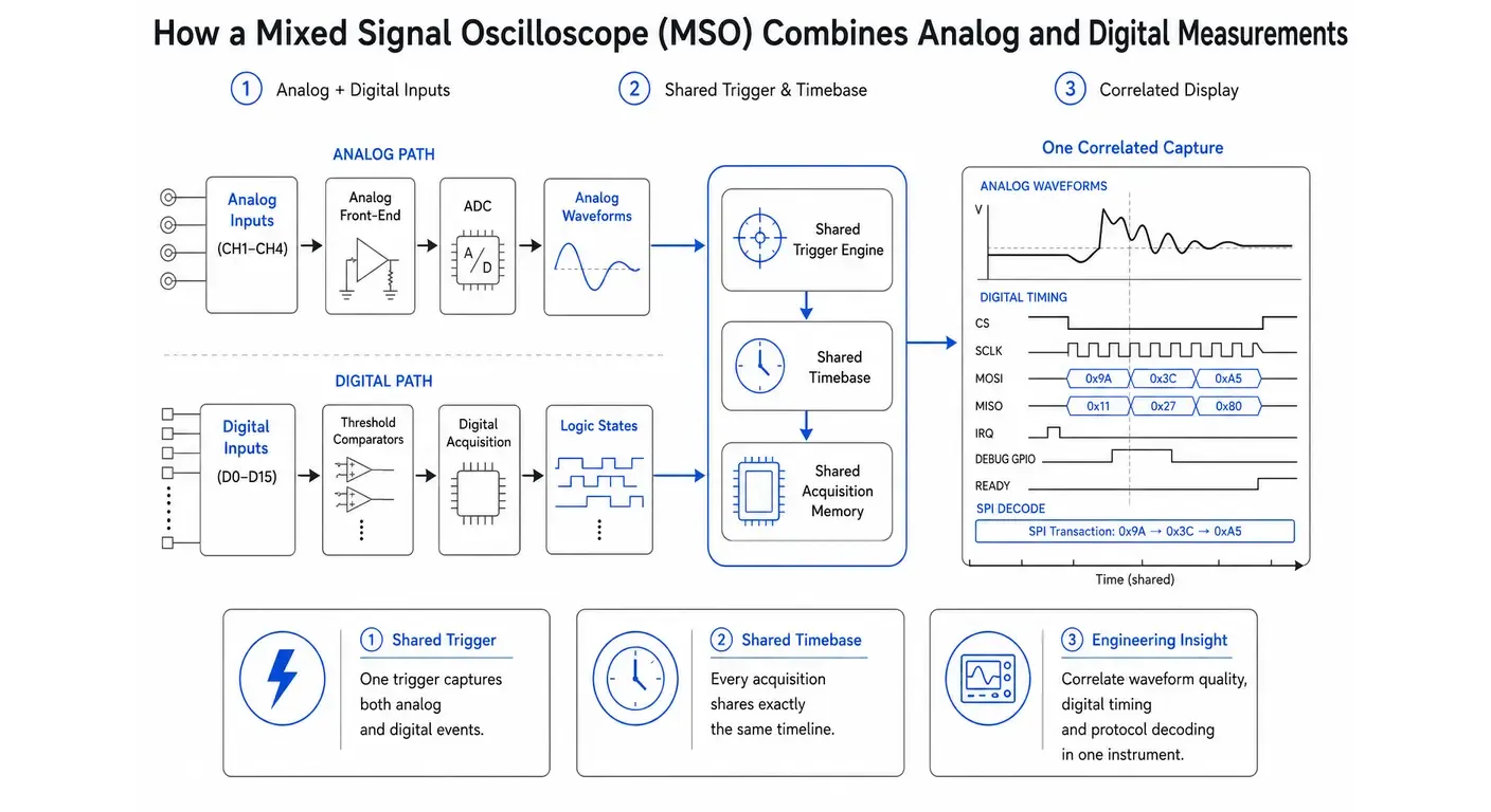
A mixed signal oscilloscope adds a set of digital channels — commonly 8 or 16 — to a conventional oscilloscope. Both acquisition paths share the same timebase, the same trigger system and the same memory management, and both appear on one screen.
Sharing the trigger is the whole point. An analog anomaly triggers the instrument and the surrounding digital bus activity is captured with it; or a decoded protocol pattern triggers the instrument and the corresponding analog waveform comes with it. Reproducing that with two separate instruments means cabling one trigger output to the other’s external trigger input — and even then the two records share no common time reference beyond the trigger event itself, so any relative timing measurement inherits the sum of both instruments’ timebase errors. Anyone who has tried to align two screenshots by eye at three in the morning understands why this feature exists.
Advantages and limitations
Pros
- Correlated analog and digital capture from a single trigger event, with both records sharing one timebase.
- One instrument, one probe setup and one user interface for mixed-signal work.
- Protocol decoding available on both analog and digital inputs, so a bus can be checked functionally and electrically without re-cabling.
- Substantially less bench space and setup time than two separate instruments.
Cons
- Digital channel count is typically 8 or 16, well below dedicated logic analyzers.
- Digital channels usually offer less capture depth and fewer advanced state-mode and sequential-trigger features than a standalone instrument.
- The digital acquisition pod is an accessory that is frequently an extra-cost option.
- Mixed-signal capability does not relax the analog bandwidth requirement — an underspecified MSO is still an underspecified oscilloscope.
Mixed signal capability is now available across the market, from cost-effective bench instruments through to portable professional instruments such as the Tektronix 2 Series MSO. The capability matters considerably more than the specific model.
Typical applications
Embedded development, motor and power control, sensor interfacing, industrial equipment maintenance, and general laboratory work where analog and digital problems arrive in roughly equal numbers. For most engineers working on microcontroller-based hardware, an MSO is the single most versatile instrument on the bench.
Choosing the Right Instrument for Your Application
Before the application-specific advice, one piece of context that explains most purchasing confusion: what actually drives cost in each instrument.
In an oscilloscope, price scales steeply with analog bandwidth. Each increment demands a faster ADC, a more linear and better-shielded front end, and every analog channel duplicates that hardware. In a logic analyzer, a channel is a comparator and a slice of memory, so channel count is cheap and price scales mainly with sample rate, capture depth and trigger sophistication.
Which is why a sixteen-channel logic analyzer frequently costs less than a single bandwidth step on an oscilloscope — and why adding a modest logic analyzer to an existing bench is usually the cheapest capability increase available to you.
Education and laboratories
Teaching laboratories benefit most from oscilloscopes, because the analog behavior of circuits is the subject being taught. A four-channel bench oscilloscope with serial decoding and reasonable memory depth covers the majority of coursework. Inexpensive USB logic analyzers can be added later at negligible cost per station.
Electronics repair
Repair work is dominated by analog questions: is the supply present, is the clock oscillating, is the signal reaching the next stage, is the waveform distorted. An oscilloscope is the primary instrument, and a logic analyzer is rarely the limiting factor.
Embedded firmware development
Firmware developers spend most of their time verifying sequences, timings and protocol behavior. A logic analyzer — from entry-level USB units through instruments such as the DreamSourceLab DSLogic or the Saleae Logic Pro series — delivers more debugging value per unit cost than almost any other tool, provided its sample rate suits the bus speeds in use. The oscilloscope remains necessary for the electrical questions firmware cannot answer.
Industrial maintenance
Field work favors portability, robustness and isolation. Handheld and portable instruments, including USB oscilloscopes such as the PicoScope series, are common, and mixed-signal capability earns its cost when PLC or drive systems combine digital control with analog process signals. Where measurements are made on mains-referenced or high-voltage circuits, correct isolation practice and appropriately rated probes are a safety requirement, not a convenience.
Research and development
R&D generally needs both capabilities at a higher performance level. On the analog side, this is where 12-bit vertical resolution earns its price: characterization work usually means resolving small perturbations on large signals — ripple on a rail, distortion in an amplifier output, a settling tail after a transient — precisely where 6 to 7 effective bits become limiting. On the digital side, high channel counts and sequential triggering matter because the fault being hunted is rare rather than obvious. An MSO frequently serves as the everyday instrument, with dedicated high-performance equipment reserved for specific investigations.
Frequently Asked Questions
Can a logic analyzer measure analog signals?
Standard logic analyzers cannot. They record only whether each input is above or below a configured threshold, so amplitude, noise and edge shape are discarded at the input comparator. A small number of instruments, such as the Saleae Logic Pro series, add dedicated analog inputs, but these sample at far lower rates and lower bandwidth than a bench oscilloscope and are best treated as a convenience rather than a replacement.
Can an oscilloscope decode SPI or I²C?
Most modern digital oscilloscopes can, either as a standard feature or as a software option. Decoding on an oscilloscope has one real advantage: it shows the electrical quality of the bus alongside the decoded data, which is exactly what you need when a protocol failure has a physical cause. The limitation is channel count and memory — an oscilloscope typically decodes one or two buses over a short capture window, while a logic analyzer decodes several over a long one.
How many channels do I need?
Count the signals that must be observed simultaneously to answer your question, then add margin. Four analog channels cover most oscilloscope work because analog investigations are usually local. Digital work is different: an SPI bus with two peripherals already needs six lines, and adding a reset, an interrupt and a firmware debug pin brings the total to nine. Sixteen digital channels is the practical baseline for embedded development.
Is a USB logic analyzer sufficient?
For low and medium speed buses it often is. The two specifications that matter are sample rate and sustained streaming throughput, because many USB instruments stream continuously to the host rather than using deep internal capture memory. That architecture means the achievable sample rate falls as more channels are enabled, and a capture can be lost entirely if the host cannot keep up. An inexpensive 24 MSa/s unit is appropriate for standard-mode I²C and typical UART traffic. Higher speed SPI, parallel buses or timing-critical measurements require a substantially higher sample rate and, ideally, internal capture memory rather than pure streaming.
Do I need both instruments?
If you work on microcontroller-based hardware, you will eventually need both measurement capabilities. Whether that means two instruments or one mixed signal oscilloscope depends on channel requirements and budget. A common and effective path is to buy the best oscilloscope the budget allows first, since it addresses problems no other instrument can, then add an inexpensive USB logic analyzer for protocol and sequencing work.
Conclusion
The comparison between an oscilloscope and a logic analyzer gets framed as a purchasing decision, but it is really a diagnostic one. The two instruments are built around opposite trade-offs: one spends its resources resolving amplitude on few channels, the other spends them resolving state on many. Each is blind in exactly the region where the other is strong.
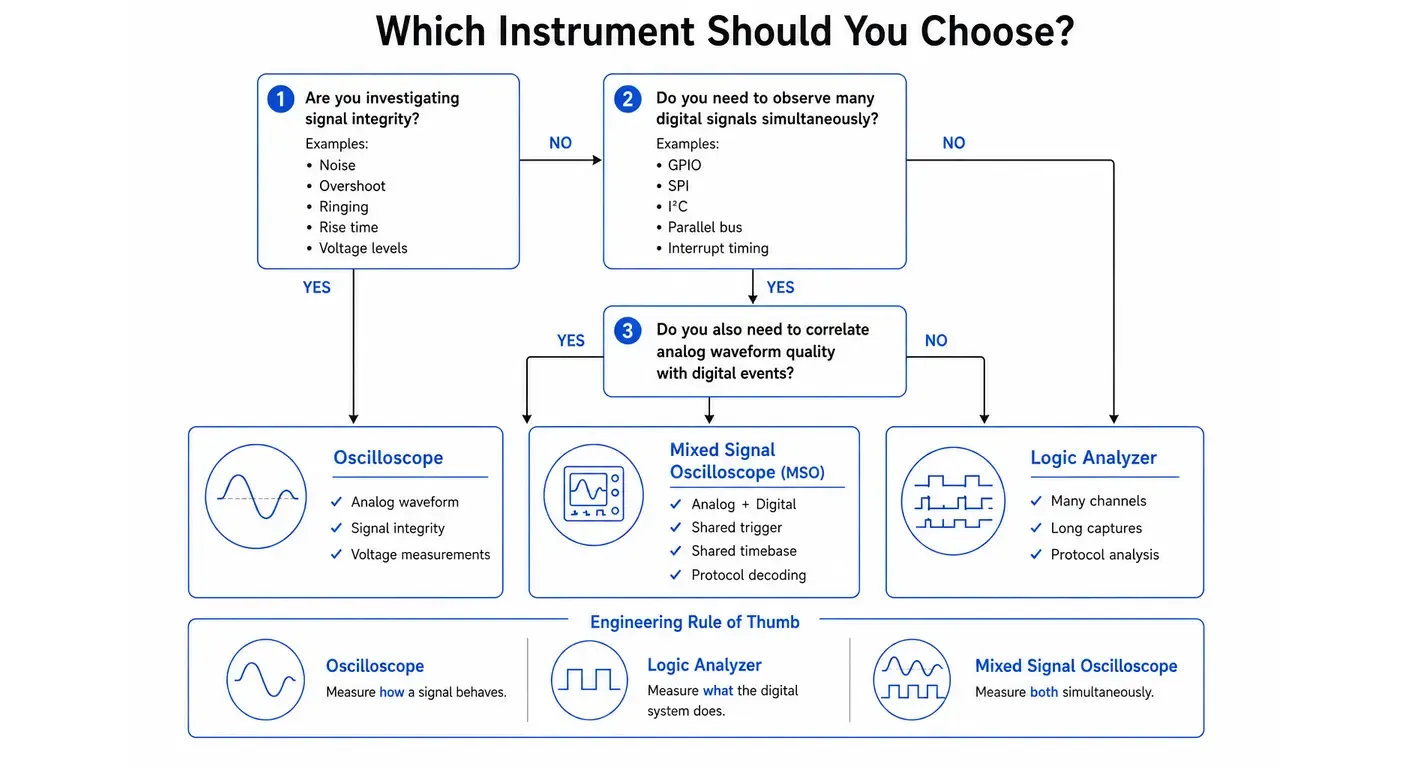
That symmetry gives you a rule you can apply at the bench. When the suspected fault concerns how a signal behaves electrically — edges, levels, noise, distortion, timing margin — reach for the oscilloscope. When it concerns what the system did — sequences, protocol content, relationships between many signals over time — reach for the logic analyzer. When the fault crosses that boundary, and in mixed-signal hardware it does so constantly, a mixed signal oscilloscope gives you both views from a single trigger.
Which brings us back to the two engineers from the opening. Neither of them chose the wrong instrument, exactly. One of them just asked a question the hardware was not answering that day.
The skill worth developing is not knowing which instrument is better. It is recognizing, before you connect anything, which question the failure is actually asking.
Related articles
Electronics18 min read
Function Generator vs Arbitrary Waveform Generator: What You Are Buying
Three names, two architectures: how DDS and point-by-point playback differ, what the labels hide, and how to read the architecture off a datasheet.
Electronics23 min read
How to Choose a Signal Generator: Getting the Signal You Asked For
How to turn a required stimulus into datasheet requirements: the load the instrument assumes, bandwidth against sample rate, reconstruction and vertical resolution.
Electronics22 min read
How to Choose a Multimeter: A Specification-Led Buying Guide
Choose a multimeter by the errors it introduces: burden voltage, input loading, AC bandwidth, safety category and accuracy on the reading you actually take.
Electronics16 min read
How to Use a Thermal Camera: Getting Readings You Can Trust
A thermal camera always shows a number. Learn the checks — emissivity, reflected temperature, focus and spot size — that decide whether it is a measurement.